MS-BioGraphs MSA10

NameMS-BioGraphs – MSA10
URLhttps://blogs.qub.ac.uk/DIPSA/MS-BioGraphs-MSA10
Download Linkhttps://doi.org/10.21227/gmd9-1534
Script for Downloading All Fileshttps://blogs.qub.ac.uk/DIPSA/MS-BioGraphs-on-IEEE-DataPort/
Validating and Sample Codehttps://blogs.qub.ac.uk/DIPSA/MS-BioGraphs-Validation/
Graph ExplanationVertices represent proteins and each edge represents the sequence similarity between its two endpoints
Edge WeightedYes
DirectedYes
Number of Vertices1,757,323,526
Number of Edges25,236,632,682
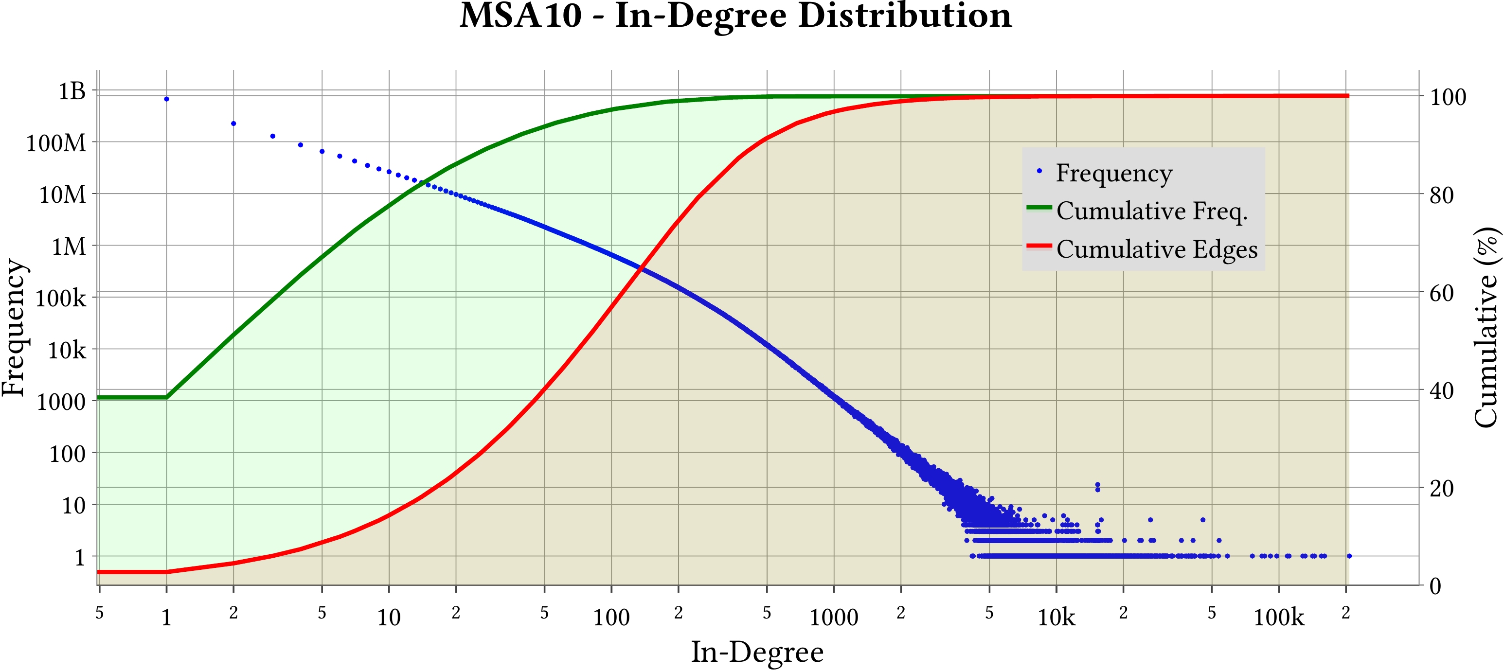
Maximum In-Degree207,279
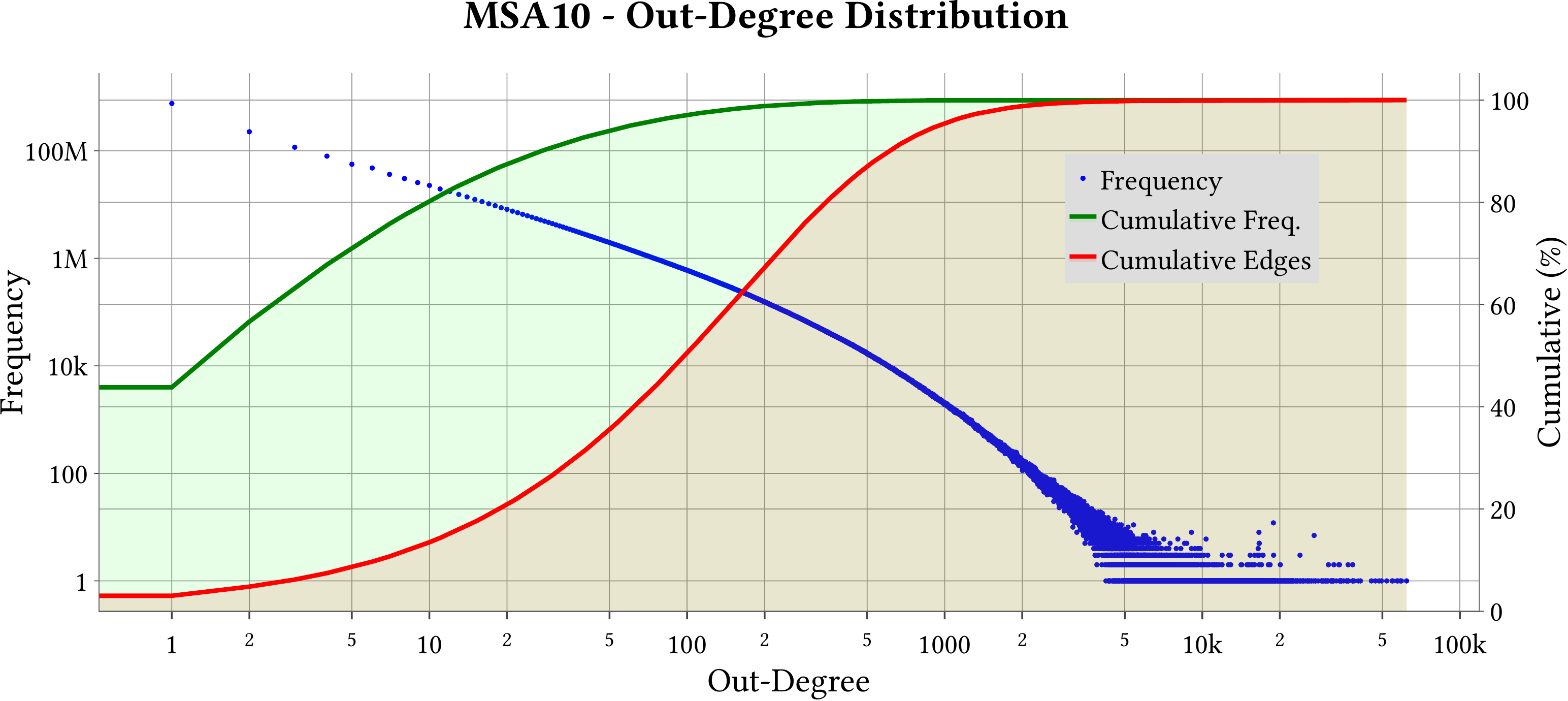
Maximum Out-Degree62,060
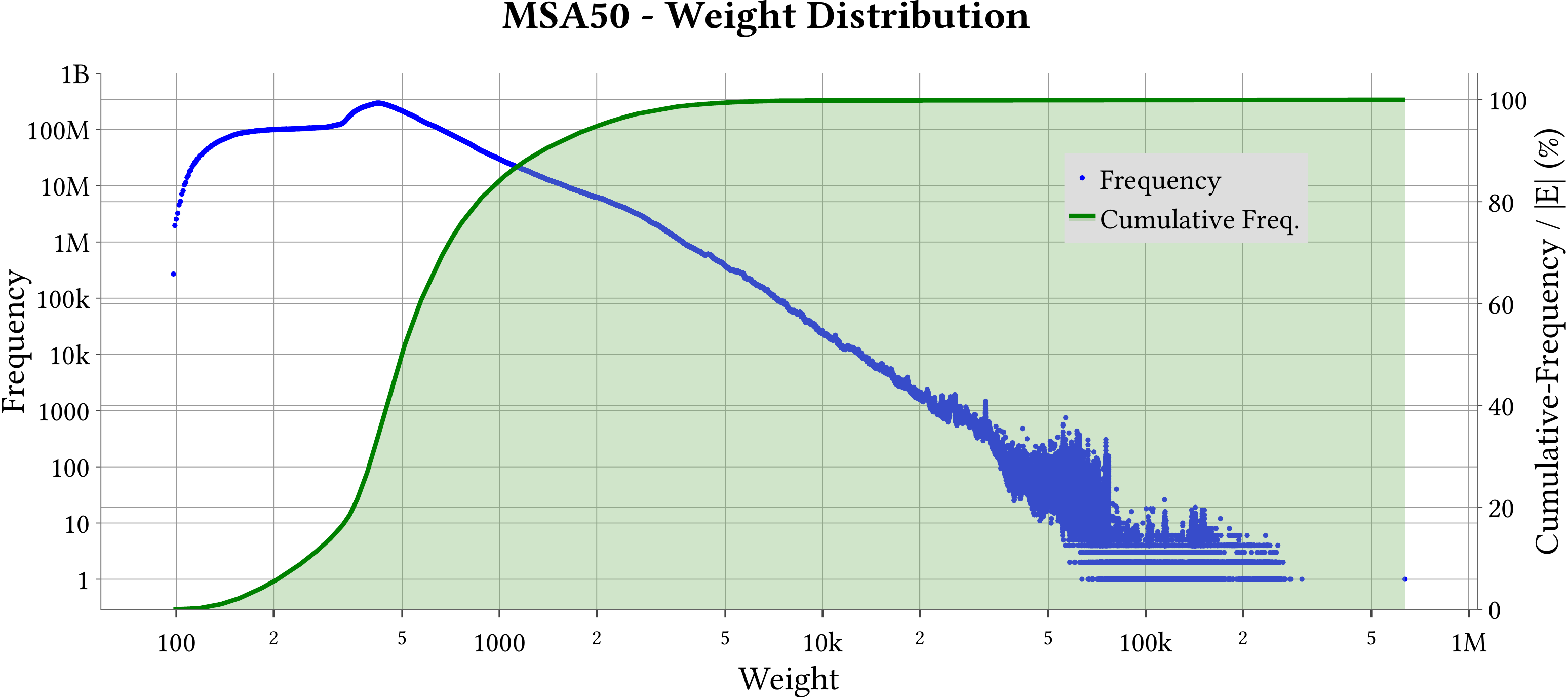
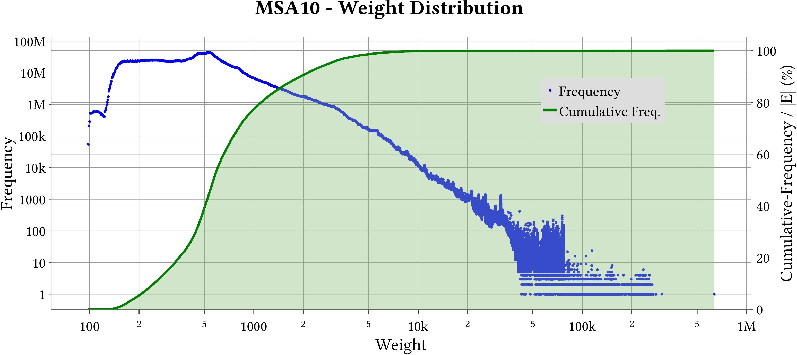
Minimum Weight98
Maximum Weight634,925
Number of Zero In-Degree Vertices6,437,984
Number of Zero Out-Degree Vertices9,926,249
Average In-Degree14.4
Average Out-Degree14.4
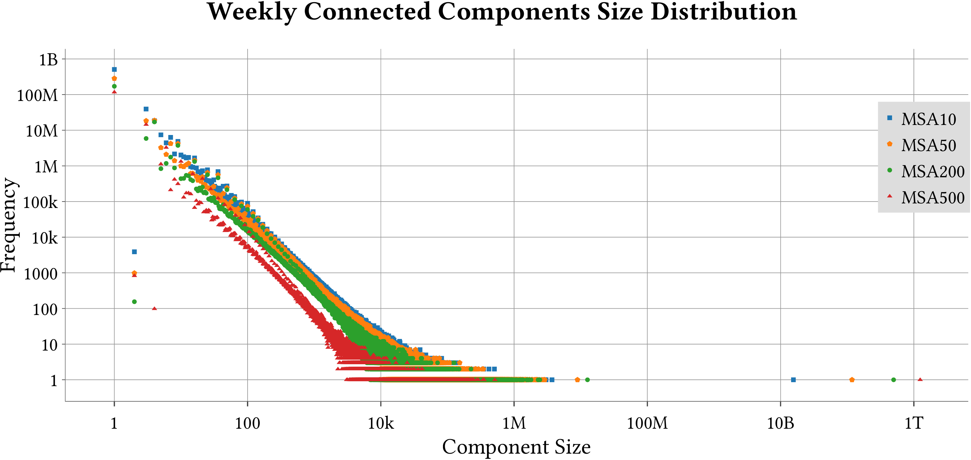
Size of The Largest Weakly Connected Component15,576,385,764
Number of Weakly Connected Components628,505,933
Creation DetailsMS-BioGraphs: Sequency Similarity Graph Datasets
FormatWebGraph
LicenseCC BY-NC-SA
QUB IDF2223-052
DOI10.5281/zenodo.7820823
Citation
Mohsen Koohi Esfahani, Sebastiano Vigna, 
Paolo Boldi, Hans Vandierendonck, Peter Kilpatrick, March 13, 2024, 
"MS-BioGraphs: Trillion-Scale Sequence Similarity Graph Datasets", 
IEEE Dataport, doi: https://doi.org/10.21227/gmd9-1534.
Bibtex
@data{gmd9-1534-24,
doi = {10.21227/gmd9-1534},
url = {https://doi.org/10.21227/gmd9-1534},
author = {Koohi Esfahani, Mohsen and Vigna, Sebastiano and Boldi, 
Paolo and Vandierendonck, Hans and Kilpatrick, Peter},
publisher = {IEEE Dataport},
title = {MS-BioGraphs: Trillion-Scale Sequence Similarity Graph Datasets},
year = {2024} }


Files

Underlying Graph The underlying graph in WebGraph format:
  • File: MSA10-underlying.graph, Size: 87,421,101,649 Bytes
  • File: MSA10-underlying.offsets, Size: 2,743,422,804 Bytes
  • File: MSA10-underlying.properties, Size: 1,439 Bytes
Total Size: 90,164,525,892 Bytes
These files are validated using ‘Edge Blocks SHAs File’ as follows.
Weights (Labels) The weights of the graph in WebGraph format:
  • File: MSA10-weights.labels, Size: 58,798,062,287 Bytes
  • File: MSA10-weights.labeloffsets, Size: 2,731,563,328 Bytes
  • File: MSA10-weights.properties, Size: 186 Bytes
Total Size: 61,529,625,801 Bytes
These files are validated using ‘Edge Blocks SHAs File’ as follows.
Edge Blocks SHAs File (Text) This file contains the shasums of edge blocks where each block contains 64 Million continuous edges and has one shasum for its 64M endpoints and one for its 64M edge weights.
The file is used to validate the underlying graph and the weights. For further explanation about validation process, please visit the https://blogs.qub.ac.uk/DIPSA/MS-BioGraphs-Validation.
  • Name: MSA10_edges_shas.txt
  • Size: 45,480 Bytes
  • SHASUM: 9c42e8ba057c519ae318071e63ab3ffdf992cd50
Offsets (Binary) The offsets array of the CSX (Compressed Sparse Rows/Columns) graph in binary format and little endian order. It consists of |V|+1 8-Bytes elements.
The first and last values are 0 and |E|, respectively.
This array helps converting the graph (or parts of it) from WebGraph format to binary format by one pass over (related) edges.
  • Name: MSA10_offsets.bin
  • Size: 14,058,588,216 Bytes
  • SHASUM: b42a8f6aee7c0abdd715f523238ea59acb09c24b
WCC (Binary) The Weakly-Connected Compontent (WCC) array in binary format and little endian order.
This array consists of |V| 4-Bytes elements The vertices in the same component have the same values in the WCC array.
  • Name: MSA10-wcc.bin
  • Size: 7,029,294,104 Bytes
  • SHASUM: 37f30d638341fa50ae9c73893e7cab689ef14be8
Transposed’s Offsets (Binary) The offsets array of the transposed graph in binary format and little endian order. It consists of |V|+1 8-Bytes elements. The first and last values are 0 and |E|, respectively.
It helps to transpose the graph by performing one pass over edges.
  • Name: MSA10_trans_offsets.bin
  • Size: 14,058,588,216 Bytes
  • SHASUM: 2ae765f6f79b8f41221ba0d869648d01d19bcadd
Names (tar.gz) This compressed file contains 120 files in CSV format using ‘;’ as the separator. Each row has two columns: ID of vertex and name of the sequence.
Note: If the graph has a ‘N2O Reordering’ file, the n2o array should be used to convert the vertex ID to old vertex ID which is used for identifying name of the protein in the `names.tar.gz` file.
  • Name: names.tar.gz
  • Size: 27,130,045,933 Bytes
  • SHASUM: ba00b58bbb2795445554058a681b573c751ef315
OJSON The charactersitics of the graph and shasums of the files.
It is in the open json format and needs a closing brace (}) to be appended before being passed to a json parser.
  • Name: MSA10.ojson
  • Size: 885 Bytes
  • SHASUM: 0d8c48f9297d36a628aabcd8576cb0c083607534


Plots

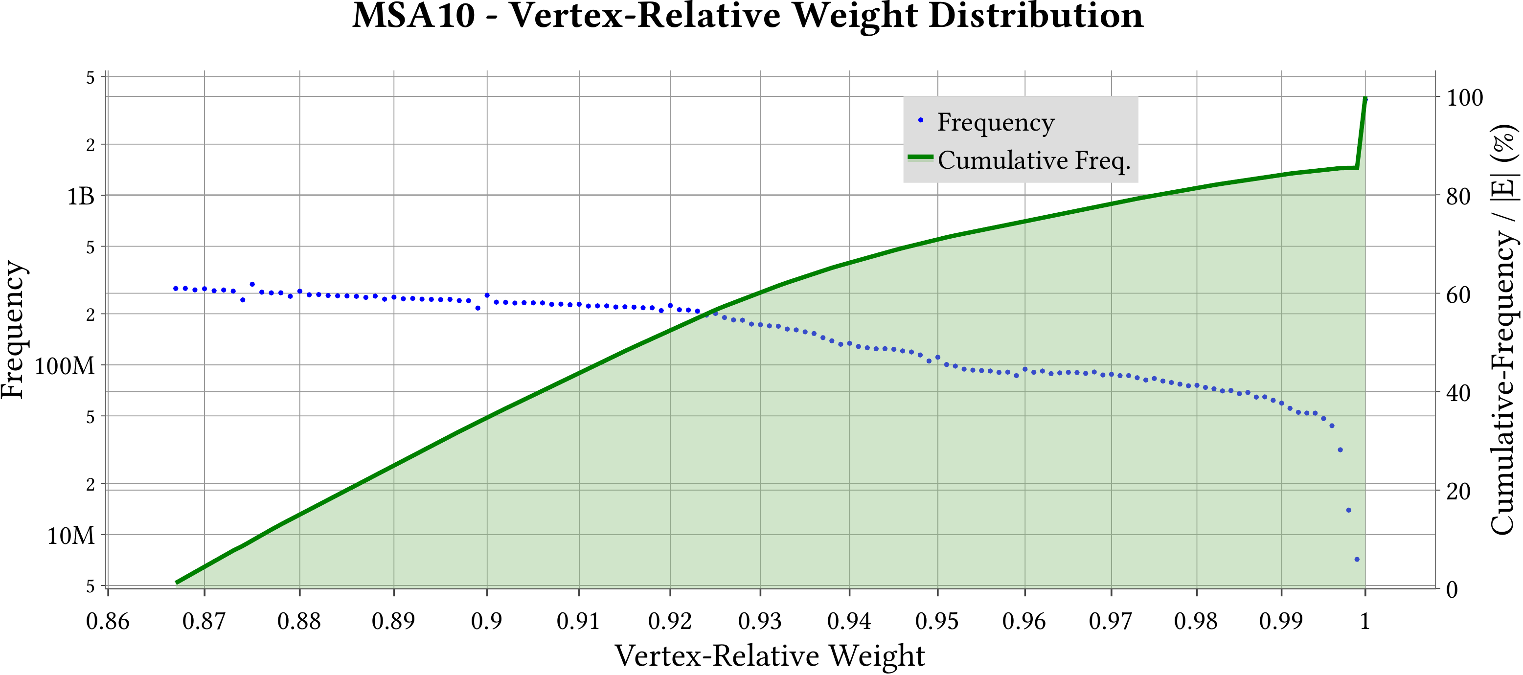
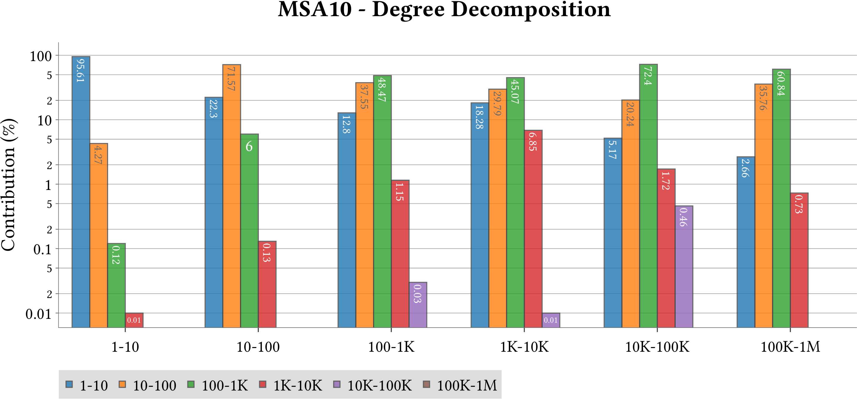
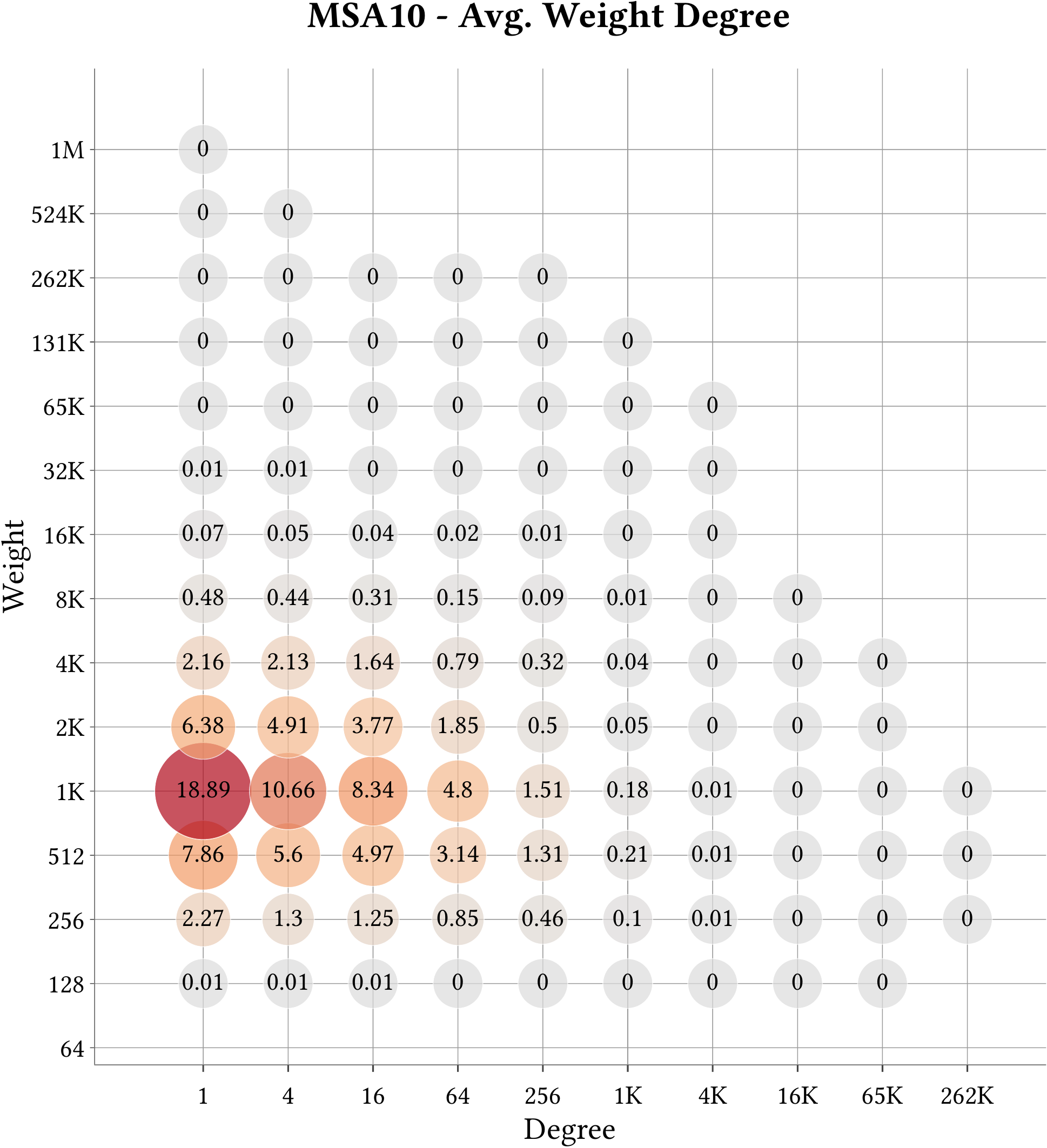
For the explanation about the plots, please refer to the MS-BioGraphs paper.
To have a better resolution, please click on the images.

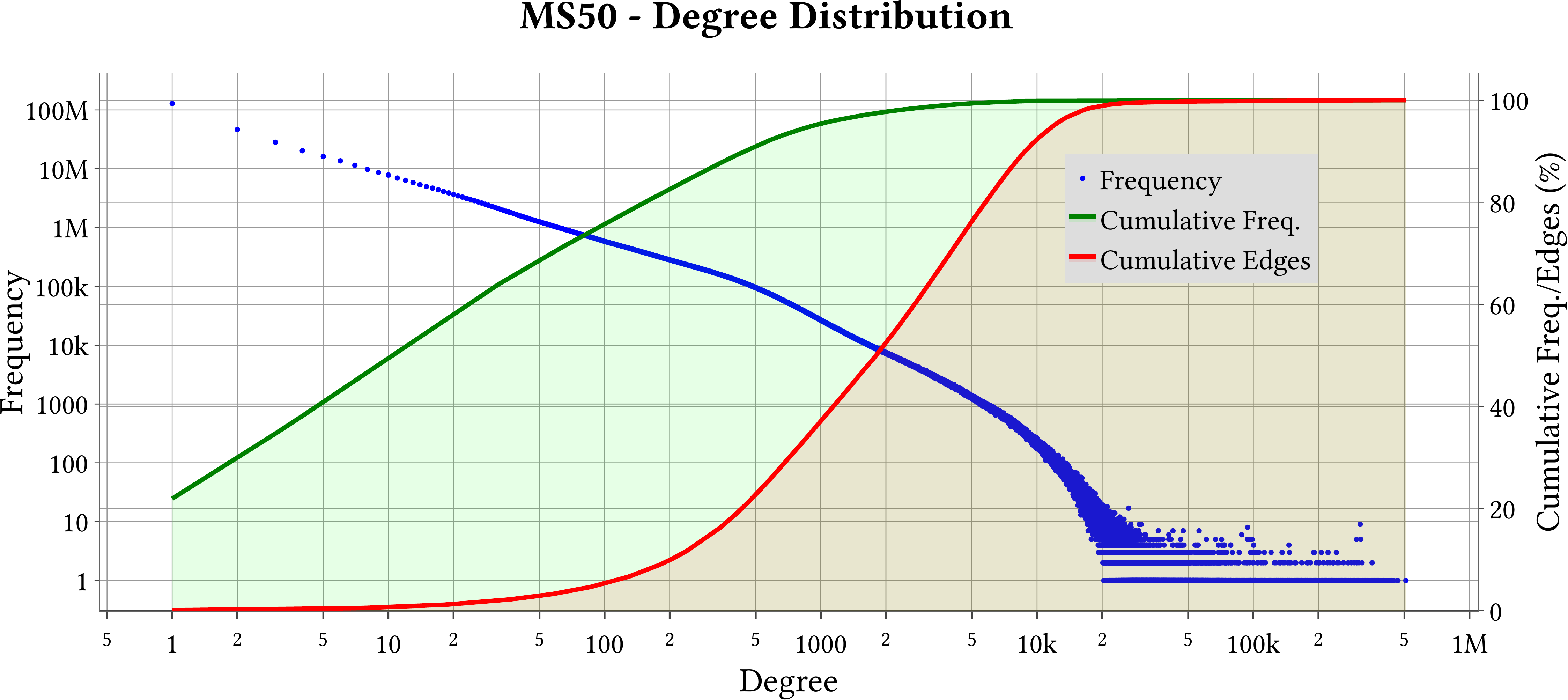
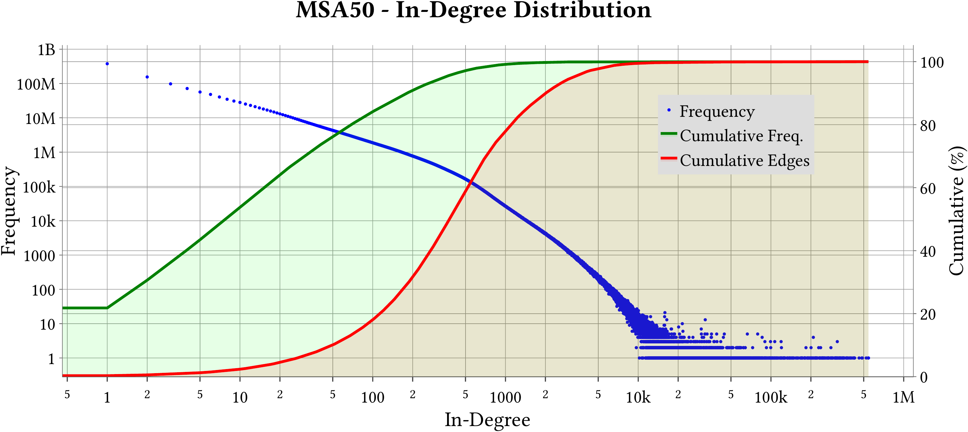
In-Degree Distribution
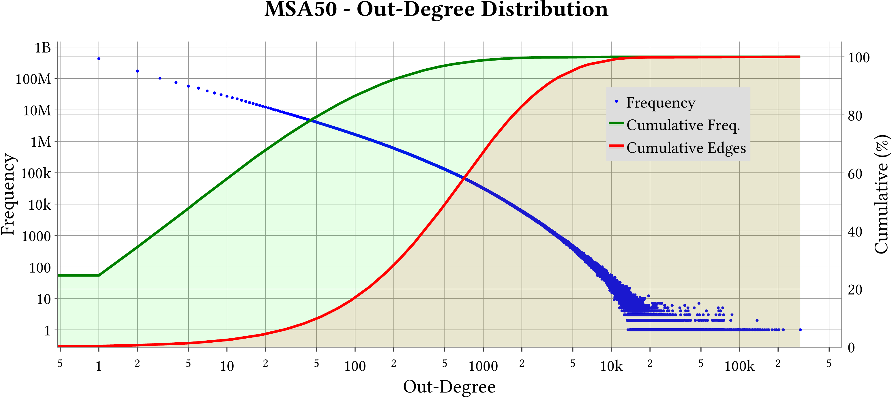
Out-Degree Distribution
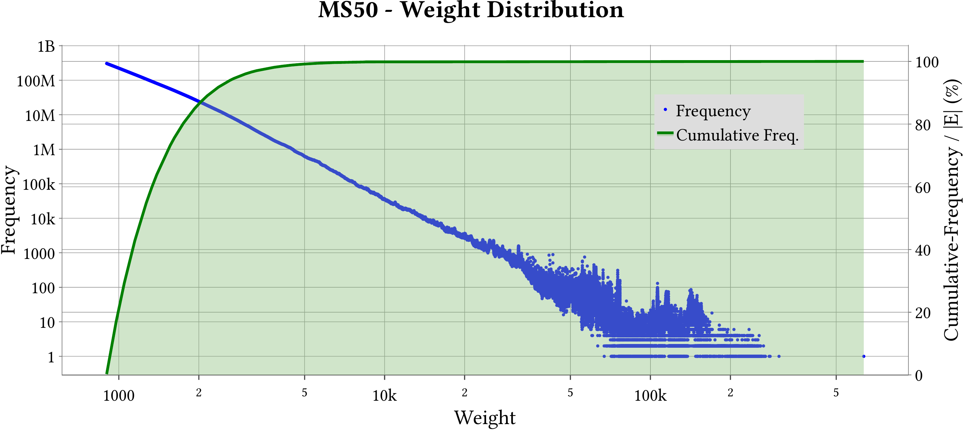
Weight Distribution
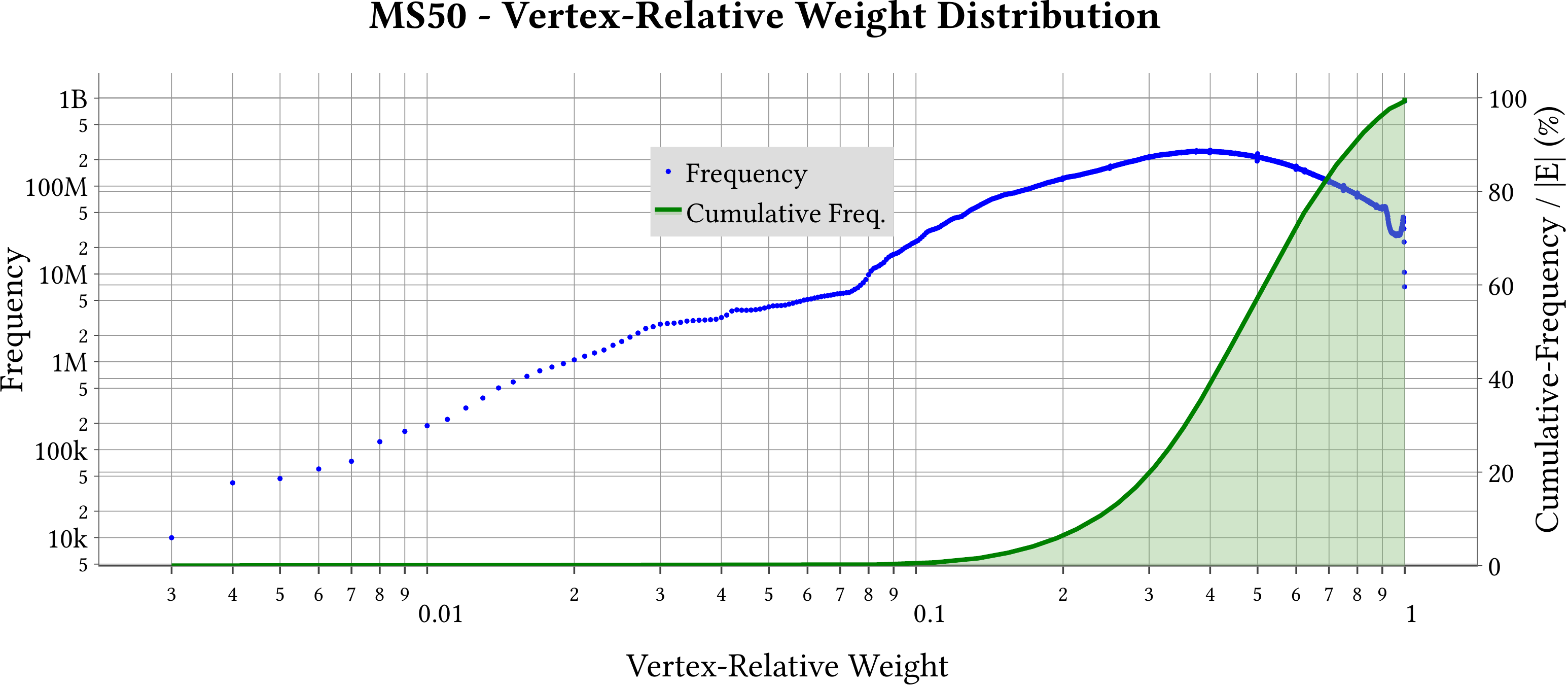
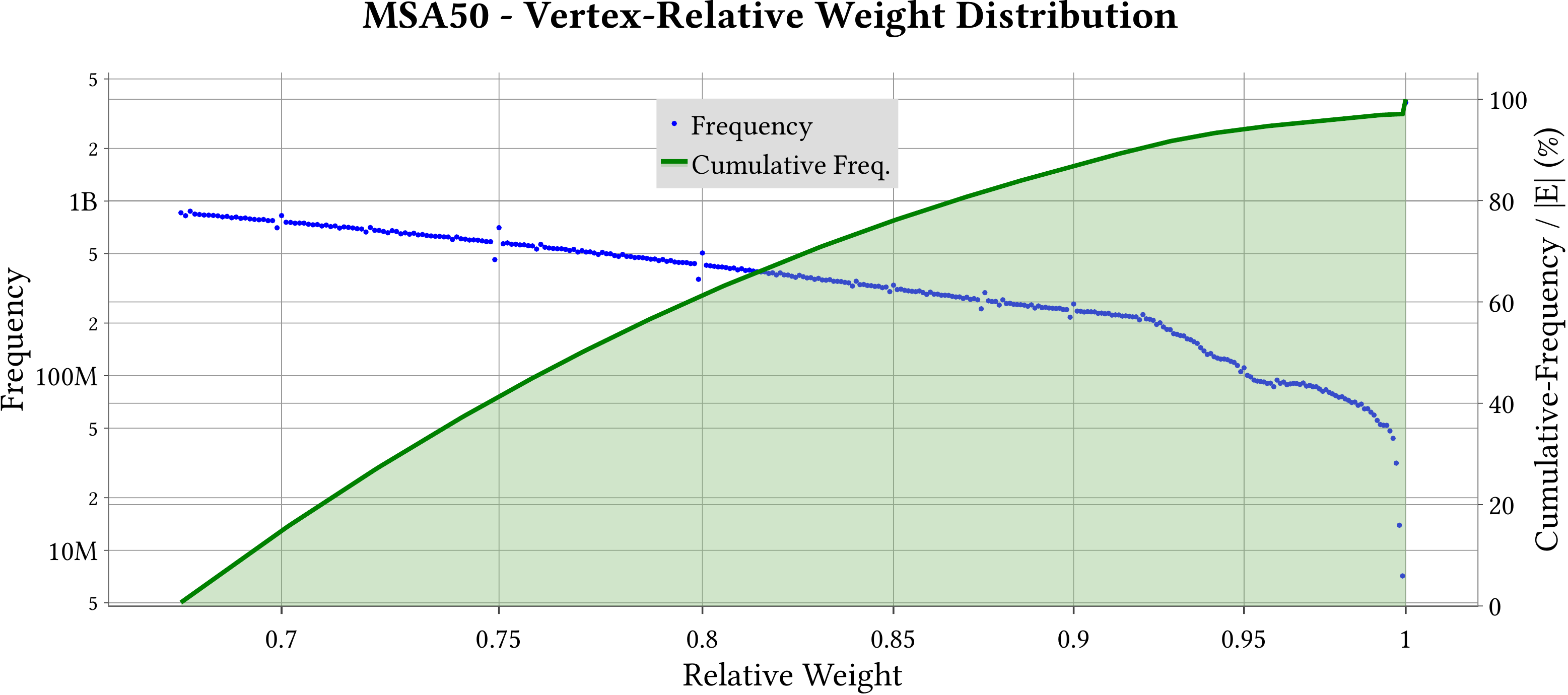
Vertex-Relative Weight Distribution
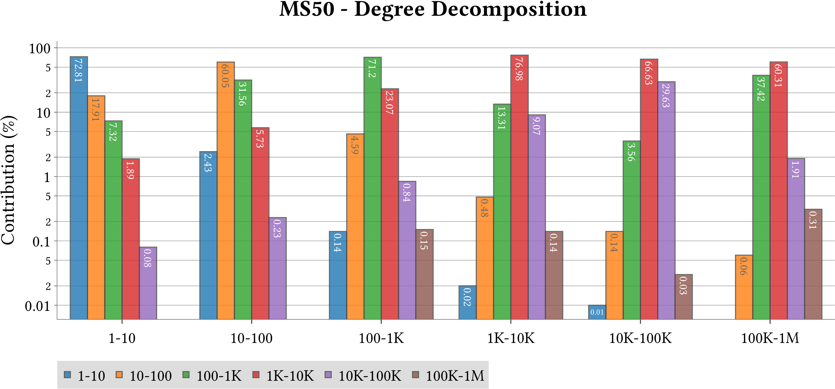
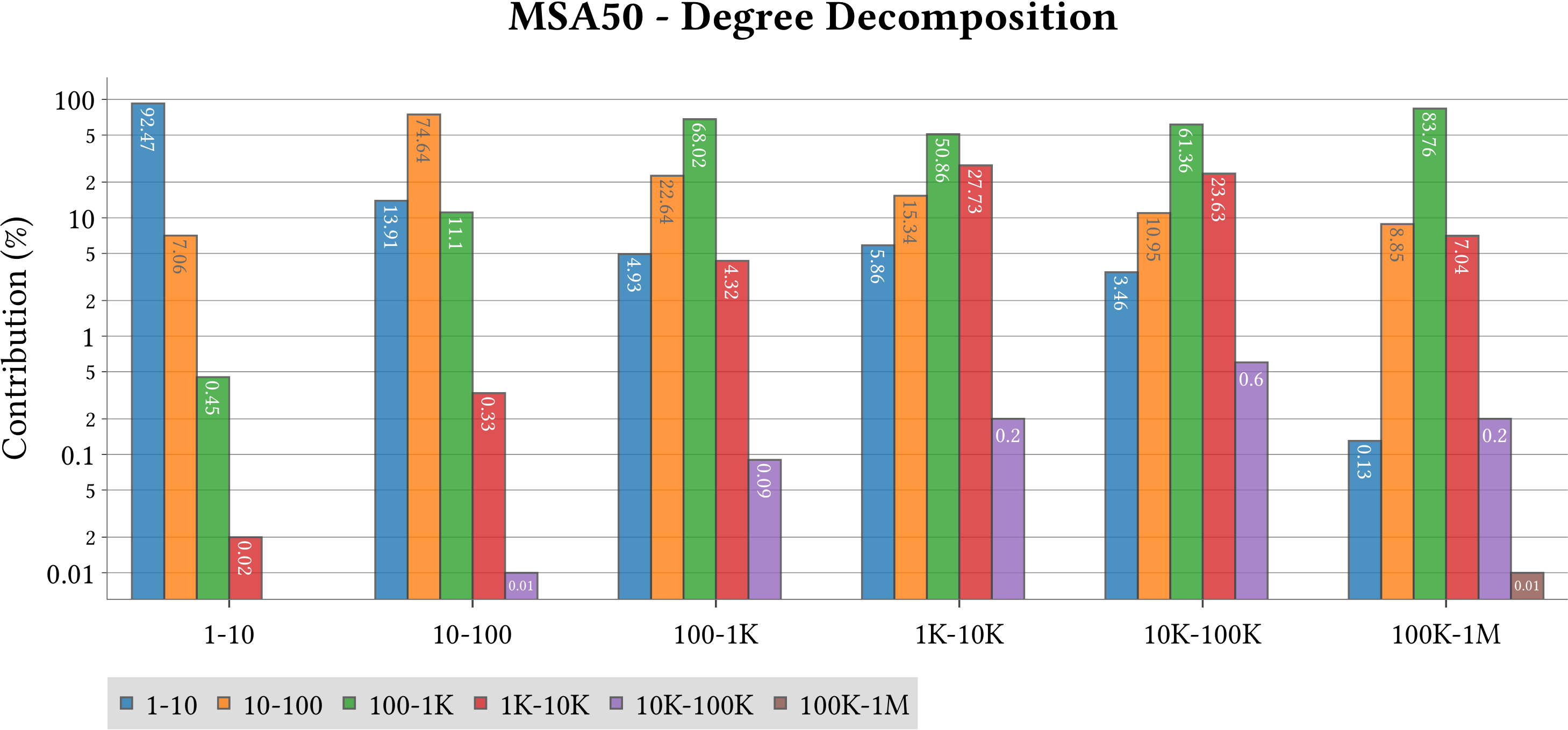
Degree Decomposition
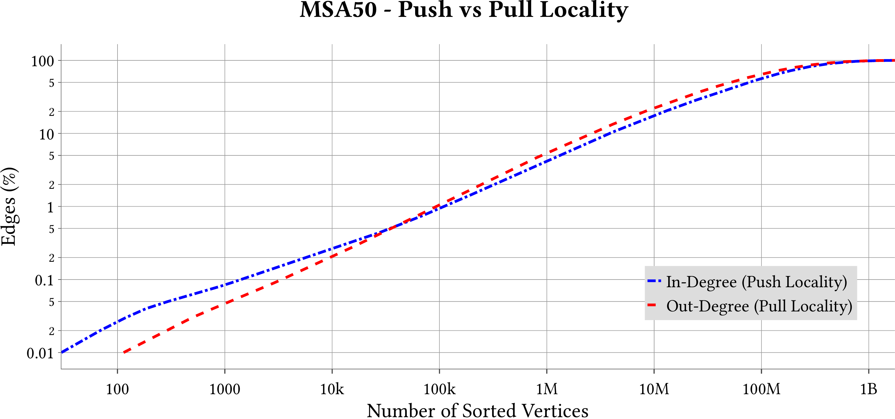
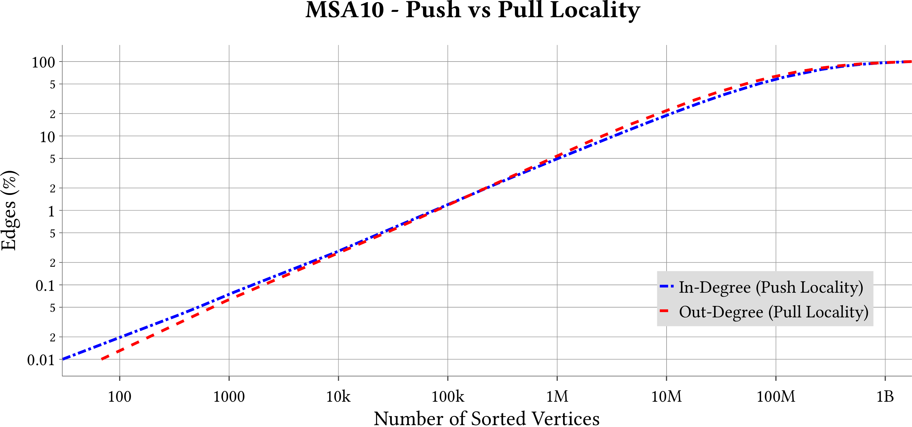
Push and Pull Locality
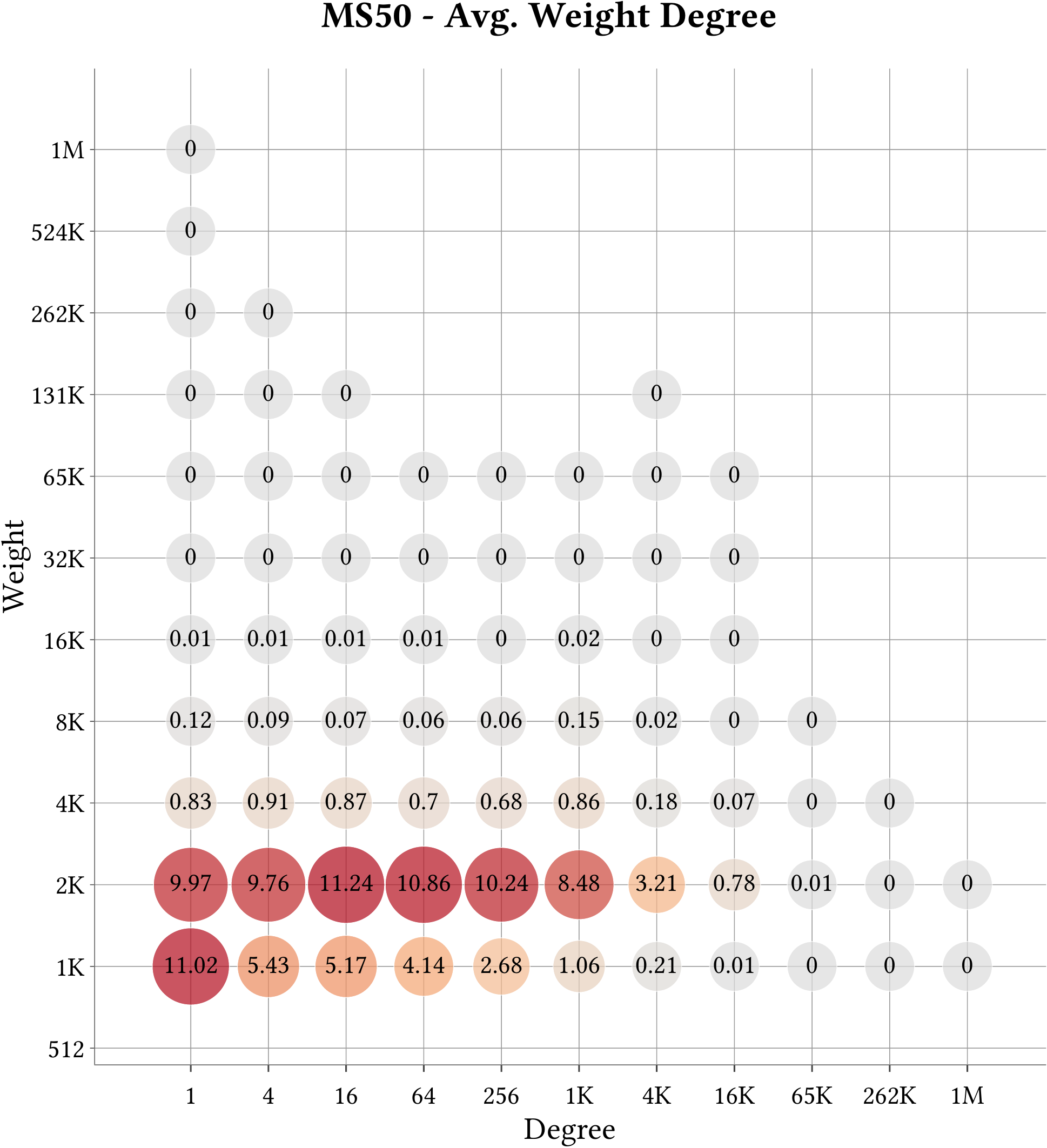
Cell-Binned Average Weight Degree Distribution
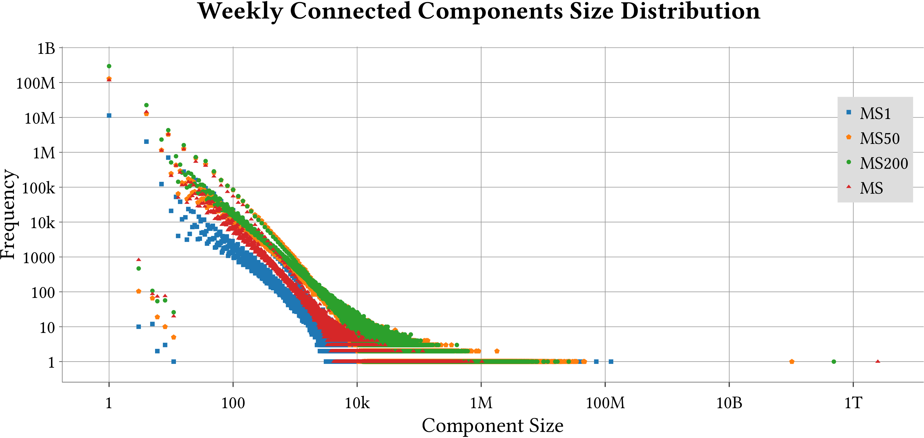
Weakly-Connected Components Size Distribution


MS-BioGraphs


Related Posts

MS-BioGraphs MS1

NameMS-BioGraphs – MS1
URLhttps://blogs.qub.ac.uk/DIPSA/MS-BioGraphs-MS1
Download Linkhttps://doi.org/10.21227/gmd9-1534
Script for Downloading All Fileshttps://blogs.qub.ac.uk/DIPSA/MS-BioGraphs-on-IEEE-DataPort/
Validating and Sample Codehttps://blogs.qub.ac.uk/DIPSA/MS-BioGraphs-Validation/
Graph ExplanationVertices represent proteins and each edge represents the sequence similarity between its two endpoints
Edge WeightedYes
DirectedNo
Number of Vertices43,144,218
Number of Edges2,660,495,200
Maximum Degree14,212
Minimum Weight3,680
Maximum Weight634,925
Number of Zero-Degree Vertices0
Average Degree61.7
Size of The Largest WCC124,003,393
Number of WCC15,746,208
Weight of Minimum Spanning Forest (ignoring self-edges)109,915,787,546
click for details
Creation DetailsMS-BioGraphs: Sequency Similarity Graph Datasets
FormatWebGraph
LicenseCC BY-NC-SA
QUB IDF2223-052
DOI10.5281/zenodo.7820827
Citation
Mohsen Koohi Esfahani, Sebastiano Vigna, 
Paolo Boldi, Hans Vandierendonck, Peter Kilpatrick, March 13, 2024, 
"MS-BioGraphs: Trillion-Scale Sequence Similarity Graph Datasets", 
IEEE Dataport, doi: https://doi.org/10.21227/gmd9-1534.
Bibtex
@data{gmd9-1534-24,
doi = {10.21227/gmd9-1534},
url = {https://doi.org/10.21227/gmd9-1534},
author = {Koohi Esfahani, Mohsen and Vigna, Sebastiano and Boldi, 
Paolo and Vandierendonck, Hans and Kilpatrick, Peter},
publisher = {IEEE Dataport},
title = {MS-BioGraphs: Trillion-Scale Sequence Similarity Graph Datasets},
year = {2024} }


Files

Underlying Graph The underlying graph in WebGraph format:
  • File: MS1-underlying.graph, Size: 6,300,911,484 Bytes
  • File: MS1-underlying.offsets, Size: 77,574,569 Bytes
  • File: MS1-underlying.properties, Size: 1,288 Bytes
Total Size: 6,378,487,341 Bytes
These files are validated using ‘Edge Blocks SHAs File’ as follows.
Weights (Labels) The weights of the graph in WebGraph format:
  • File: MS1-weights.labels, Size: 8,201,441,365 Bytes
  • File: MS1-weights.labeloffsets, Size: 80,797,007 Bytes
  • File: MS1-weights.properties, Size: 184 Bytes
Total Size: 8,282,238,556 Bytes
These files are validated using ‘Edge Blocks SHAs File’ as follows.
Edge Blocks SHAs File (Text) This file contains the shasums of edge blocks where each block contains 64 Million continuous edges and has one shasum for its 64M endpoints and one for its 64M edge weights.
The file is used to validate the underlying graph and the weights. For further explanation about validation process, please visit the https://blogs.qub.ac.uk/DIPSA/MS-BioGraphs-Validation.
  • Name: MS1_edges_shas.txt
  • Size: 5,040 Bytes
  • SHASUM: 27974edb4bf8f3b17b00ff3a72a703da18f3807a
Offsets (Binary) The offsets array of the CSX (Compressed Sparse Rows/Columns) graph in binary format and little endian order. It consists of |V|+1 8-Bytes elements.
The first and last values are 0 and |E|, respectively.
This array helps converting the graph (or parts of it) from WebGraph format to binary format by one pass over (related) edges.
  • Name: MS1_offsets.bin
  • Size: 345,153,752 Bytes
  • SHASUM: 0abedde32e1ac7181897f82d10d40acfe14f2022
WCC (Binary) The Weakly-Connected Compontent (WCC) array in binary format and little endian order.
This array consists of |V| 4-Bytes elements The vertices in the same component have the same values in the WCC array.
  • Name: MS1-wcc.bin
  • Size: 172,576,872 Bytes
  • SHASUM: 4c491dd96e3582b70a203ae4a910001381278d75
Names (tar.gz) This compressed file contains 120 files in CSV format using ‘;’ as the separator. Each row has two columns: ID of vertex and name of the sequence.
Note: If the graph has a ‘N2O Reordering’ file, the n2o array should be used to convert the vertex ID to old vertex ID which is used for identifying name of the protein in the `names.tar.gz` file.
  • Name: names.tar.gz
  • Size: 27,130,045,933 Bytes
  • SHASUM: ba00b58bbb2795445554058a681b573c751ef315
N2O Reordering (Binary) The New to Old (N2O) reordering array of the graph in binary format and little endian order.
It consists of |V| 4-Bytes elements and identifies the old ID of each vertex which is used in searching the name of vertex (protein) in the names.tar.gz file .
  • Name: MS1-n2o.bin
  • Size: 172,576,872 Bytes
  • SHASUM: b163320b6349fed7a00fb17c4a4a22e7d124b716
OJSON The charactersitics of the graph and shasums of the files.
It is in the open json format and needs a closing brace (}) to be appended before being passed to a json parser.
  • Name: MS1.ojson
  • Size: 736 Bytes
  • SHASUM: c60afa0652955fd46f1bb8056380523504d69fa6


Plots

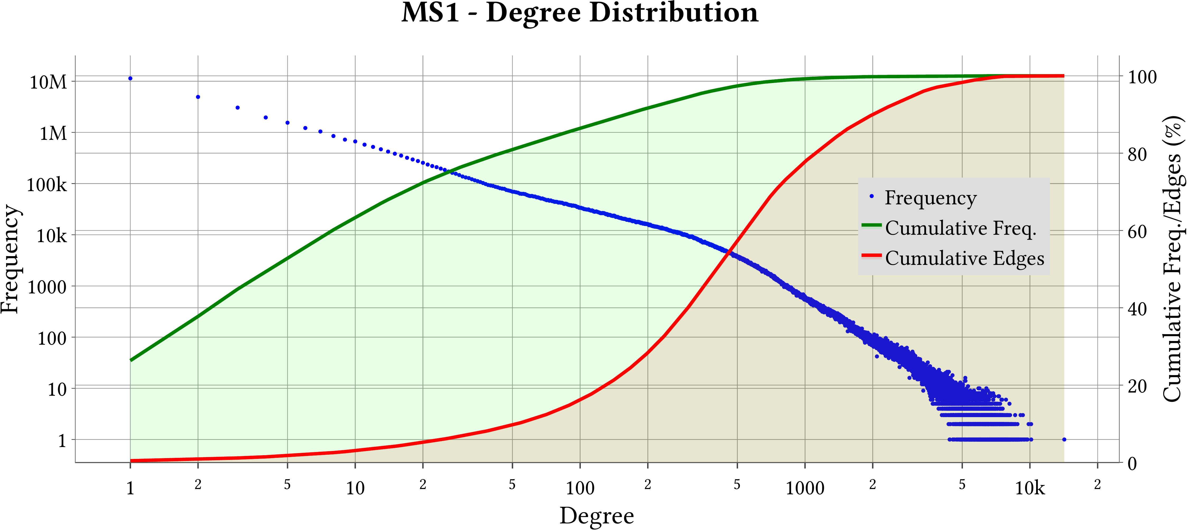
For the explanation about the plots, please refer to the MS-BioGraphs paper.
To have a better resolution, please click on the images.

Degree Distribution
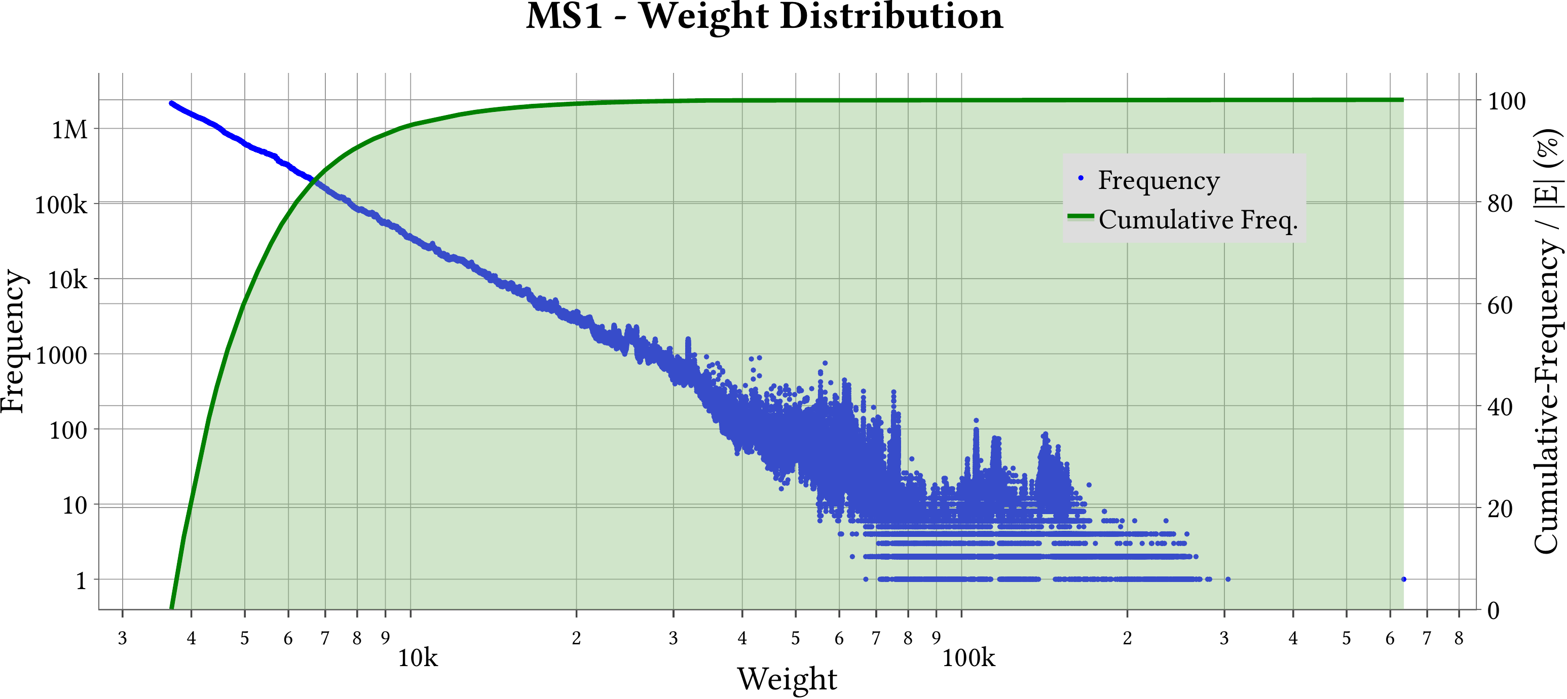
Weight Distribution
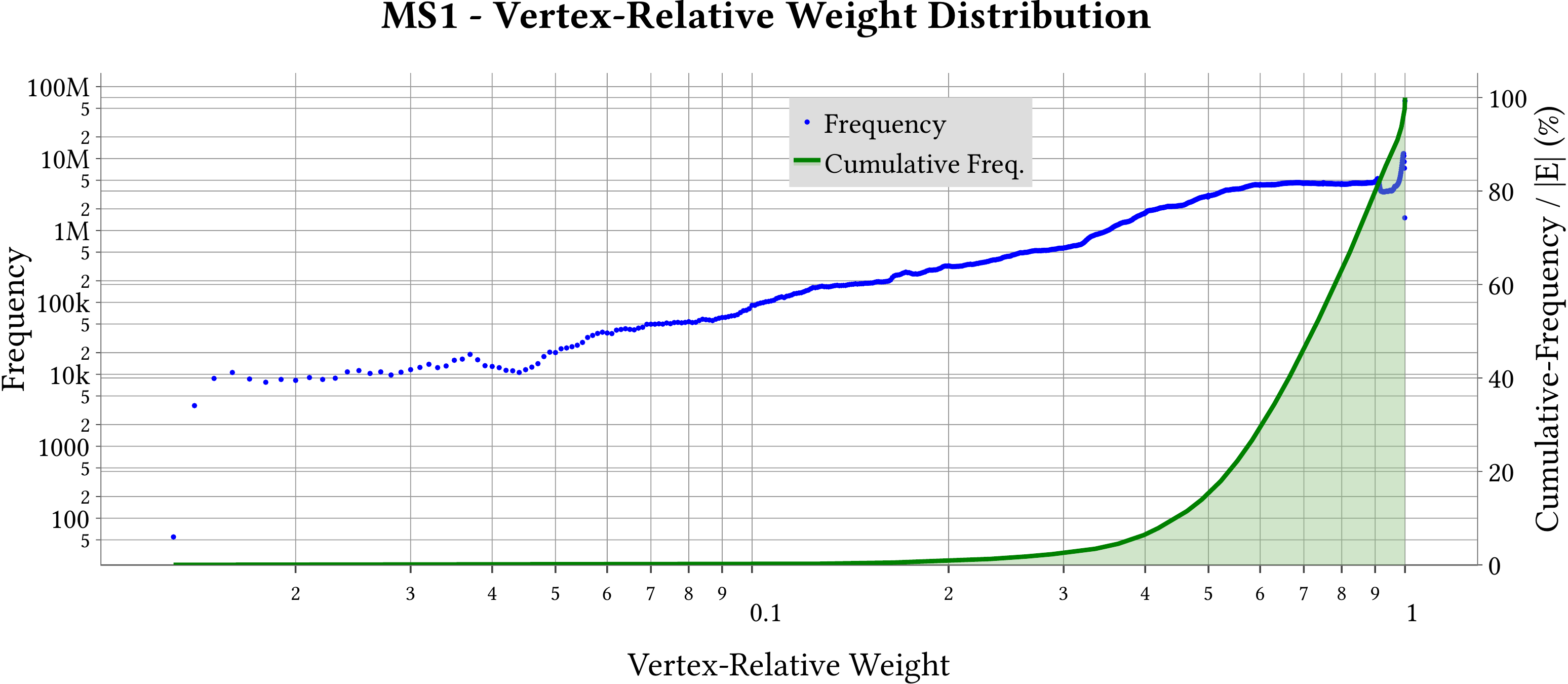
Vertex-Relative Weight Distribution
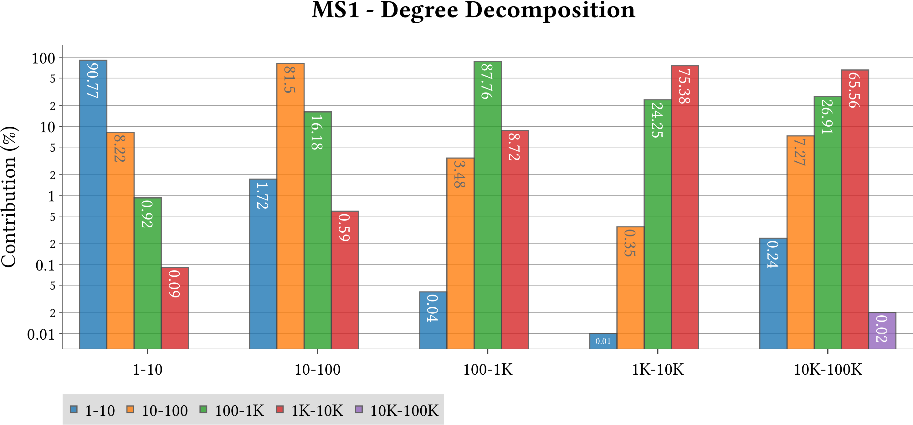
Degree Decomposition
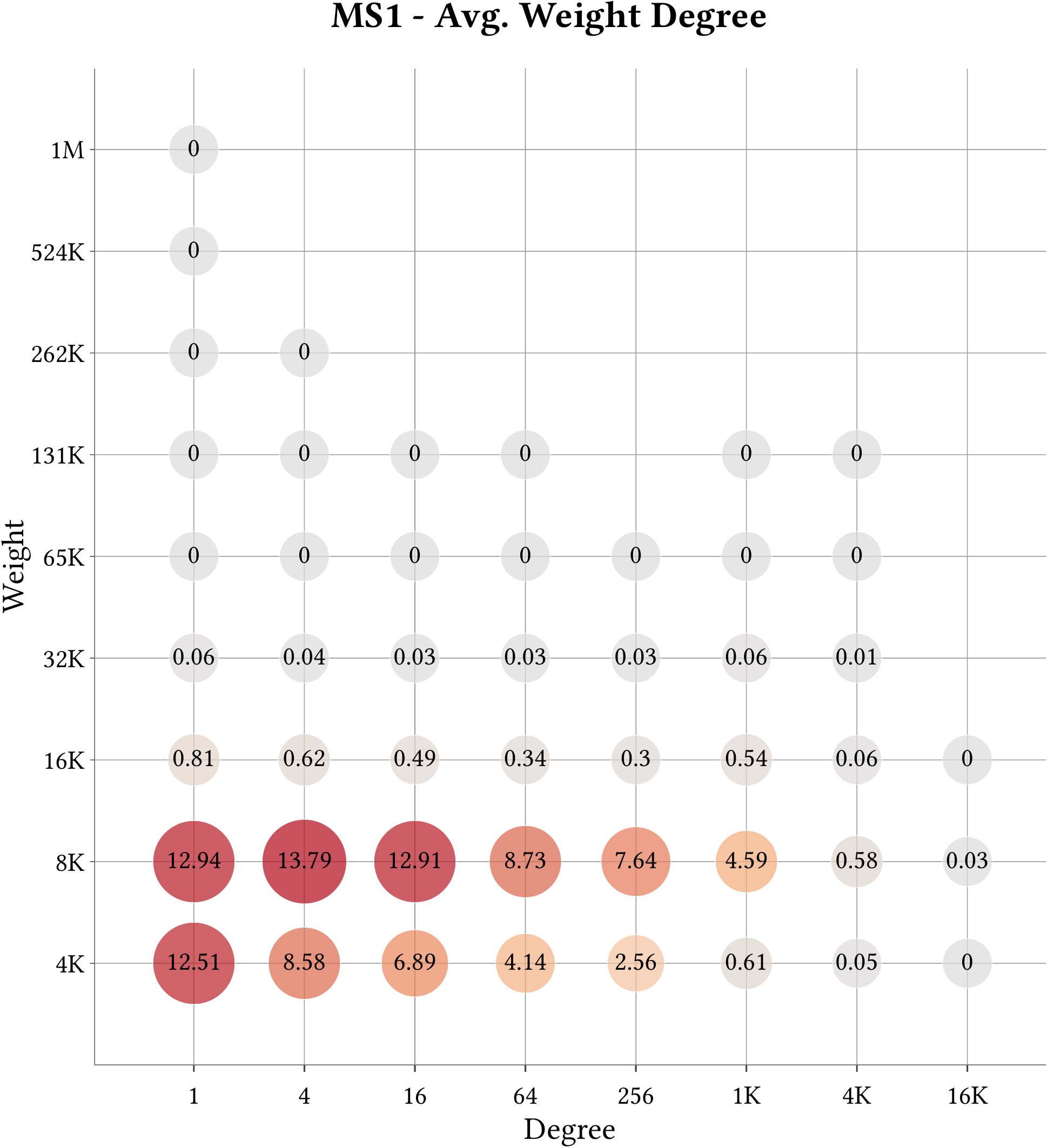
Cell-Binned Average Weight Degree Distribution
Weakly-Connected Components Size Distribution


MS-BioGraphs


Related Posts

MS-BioGraphs Validation
Repository

https://github.com/DIPSA-QUB/MS-BioGraphs-Validation

Explanation

We provide a Shell script, validation.sh, and a Java program, EdgeBlockSHA.java, to verify the the correctness of the graphs. Each graph has a .ojson file whose shasum is verified by the value retreived from our server. Files such as offsets.bin, wcc.bin, n2o.bin, trans_offsets.bin, and edges_shas.txt have shasum records in the ojson file which is used for validation of these files.

The graph in WebGraph format has been compressed in MS??-underlying.* and MS??-weights.* files. In order to validate the compressed graph, the EdgeBlockSHA.java is used. It is a parallel Java code that uses the WebGraph library to traverse the graph and calculate the shasum of blocks of edges (endpoints and weights). Then, the calculated results are matched with the edges_shas.txt file of the graph.

It is also possible to validate some particular blocks by matching the calculated shasum with the relevant row in the edges_shas.txt file. This file has a format such as the following. Each block contains 64 Million consecutive edges. The start of each block is identified by a vertex ID and its edge index. The Column endpoint_sha is the shasum of the 64 Million endpoints when stored as an array of 4-Bytes elements in the binary format and in the little endian order. Similarly, Column weights_sha shows the shasum of weights (labels). We have separated weights from endpoints as in some applications weights are not needed and therefore it is not necessary to read and validate them.

64MB blk#;     vertex; edge index;                             endpoint_sha;                              weights_sha;
         0;          0;          0; 509784b158cb9404241afb21d0ceaf590b88d2f2; 57da4ad7bb89c5922e436b0535d791fa8f40dffd;
         1;    2315113;        705; fafc118563c1d7b5fbff64af56edd6a56524f479; 13b7a9ca60bfb0715d563218d0a1cd787b00a07c;
         2;    4521625;        597; 4ed65aa07c8062a151166ef2e9bdb93e41d19357; 8158276bec426ee46eca9912759eb9bd57fcc957;
         3;    6347361;        112; d02e8913c807c3f4ecde9c638e0ded5ab80ba819; 26bc3296de65cba6ac539cd96b79ae6f7a4d37be;
         4;    8447869;         15; 61513c84db40124496cdf769516118b63598914f; 781b9f4372ac614e94d097017c756d015234deb6; 
 

Requirements

  • JDK with version > 15
  • jq
  • wget

WebGraph Framework

Please visit https://webgraph.di.unimi.it .

ParaGrapher Graph Loading API and Library

The WebGraph formats can also be read using the ParaGrapher library: https://blogs.qub.ac.uk/DIPSA/ParaGrapher/.

License

Licensed under the GNU v3 General Public License, as published by the Free Software Foundation. You must not use this Software except in compliance with the terms of the License. Unless required by applicable law or agreed upon in writing, this Software is distributed on an “as is” basis, without any warranty; without even the implied warranty of merchantability or fitness for a particular purpose, neither express nor implied.

Copyright 2022-2023 The Queen’s University of Belfast, Northern Ireland, UK

MS-BioGraphs

Related Posts

On Designing Structure-Aware High-Performance Graph Algorithms (PhD Thesis)

Mohsen Koohi Esfahani
Supervisors: Hans Vandierendonck and Peter Kilpatrick

Thesis in PDF format
Thesis on QUB Pure Portal

Graph algorithms find several usages in industry, science, humanities, and technology. The fast-growing size of graph datasets in the context of the processing model of the current hardware has resulted in different bottlenecks such as memory locality, work-efficiency, and load-balance that degrade the performance. To tackle these limitations, high-performance computing considers different aspects of the execution in order to design optimized algorithms through efficient usage of hardware resources.

The main idea in this thesis is to analyze the structure of graphs to exploit special features that are key to introduce new graph algorithms with optimized performance.

First, we study the structure of real-world graph datasets with skewed degree distribution and the applicability of graph relabeling algorithms as the main restructuring tools to improve performance and memory locality. To that end, we introduce novel locality metrics including Cache Miss Rate Degree Distribution, Effective Cache Size, Push Locality and Pull Locality, and Degree Range Decomposition.

Based on this structural analysis, we introduce the Uniform Memory Demands strategy that (i) recognizes diverse memory demands and behaviours as a source of performance inefficiency, (ii) separates contrasting memory demands into groups with uniform behaviours across each group, and (iii) designs bespoke data structures and algorithms for each group in order to satisfy memory demands with the lowest overhead.

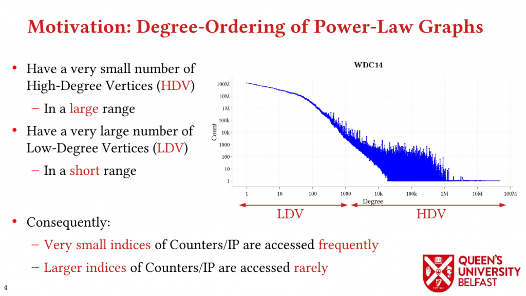
We apply the Uniform Memory Demands strategy to design three graph algorithms with optimized performance: (i) the SAPCo Sort algorithm as a parallel counting sort algorithm that is faster than comparison-based sorting algorithms in degree-ordering of power-law graphs, (ii) the iHTL algorithm that optimizes locality in Sparse Matrix-Vector (SpMV) Multiplication graph algorithms by extracting dense subgraphs containing incoming edges to in-hubs and processing them in the push direction, and (iii) the LOTUS algorithm that optimizes locality in Triangle Counting by separating different caching demands and deploying specific data structure and algorithm for each of them.

Bibtex

@phdthesis{ODSAGA-ethos.874822,
  title  = {On Designing Structure-Aware High-Performance Graph Algorithms},
  author = {Mohsen Koohi Esfahani},
  year   = 2022,
  url    = {https://blogs.qub.ac.uk/DIPSA/On-Designing-Structure-Aware-High-Performance-Graph-Algorithms-PhD-Thesis/},
  school = {Queen's University Belfast},
  EThOSID = {uk.bl.ethos.874822}
}

Related Posts

LaganLighter

LaganLighter Source Code


Repository

https://github.com/DIPSA-QUB/LaganLighter

Documentation
https://github.com/DIPS-QUB/LaganLighter/tree/main/docs

Algorithms in This Repo

Cloning

git clone https://github.com/MohsenKoohi/LaganLighter.git --recursive

Graph Types

LaganLighter supports the following graph formats:

  • CSR/CSC graph in text format, for testing. This format has 4 lines: (i) number of vertices (|V|), (ii) number of edges (|E|), (iii) |V| space-separated numbers showing offsets of the vertices, and (iv) |E| space-separated numbers indicating edges.
  • CSR/CSC WebGraph format: supported by the Poplar Graph Loading Library
    external git repository

Measurements

In addition to execution time, we use the PAPI library to measure hardware counters such as L3 cache misses, hardware instructions, DTLB misses, and load and store memory instructions. ( papi_(init/start/reset/stop) and (print/reset)_hw_events functions defined in omp.c).
To measure load balance, we measure the total time of executing a loop and the time each thread spends in this loop (mt and ttimes in the following sample code). Using these values, PTIP macro (defined in omp.c) calculates the percentage of average idle time (as an indicator of load imbalance) and prints it with the total time (mt).

mt = - get_nano_time()
#pragma omp parallel  
{
   unsigned tid = omp_get_thread_num();
   ttimes[tid] = - get_nano_time();
	
   #pragma omp for nowait
   for(unsigned int v = 0; v < g->vertices_count; v++)
   {
      // .....
   }
   ttimes[tid] += get_nano_time();
}
mt += get_nano_time();
PTIP("Step ... ");

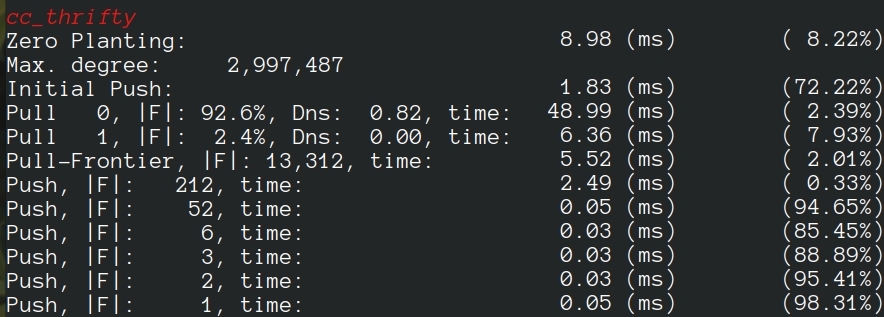
As an example, the following execution of Thrifty, shows that the “Zero Planting” step has been performed in 8.98 milliseconds and with a 8.22% load imbalance, while processors have been idle for 72.22% of the execution time, on average, in the “Initial Push” step.

NUMA-Aware and Locality-Preserving Partitioning and Scheduling

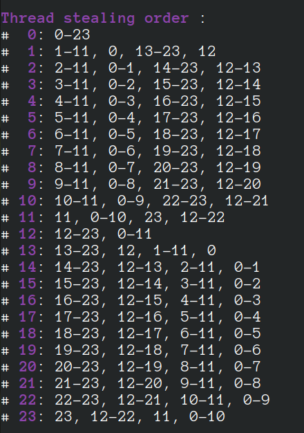
In order to assign consecutive partitions (vertices and/or their edges) to each parallel processor, we initially divide partitions and assign a number of consecutive partitions to each thread. Then, we specify the order of victim threads in the work-stealing process. During the initialization of LaganLighter parallel processing environment (in initialize_omp_par_env() function defined in file omp.c), for each thread, we create a list of threads as consequent victims of stealing.

A thread, first, steals jobs (i.e., partitions) from consequent threads in the same NUMA node and then from the threads in consequent NUMA nodes. As an example, the following image shows the stealing order of a 24-core machine with 2 NUMA nodes. This shows that thread 1 steals from threads 2, 3, …,11, and ,0 running on the same NUMA socket and then from threads 13, 14, …, 23, and 12 running on the next NUMA socket.

We use dynamic_partitioning_...() functions (in file partitioning.c) to process partitions by threads in the specified order. A sample code is in the following:

struct dynamic_partitioning* dp = dynamic_partitioning_initialize(pe, partitions_count);

#pragma omp parallel  
{
   unsigned int tid = omp_get_thread_num();
   unsigned int partition = -1U;		

   while(1)
   {
      partition = dynamic_partitioning_get_next_partition(dp, tid, partition);
      if(partition == -1U)
	 break; 

      for(v = start_vertex[partition]; v < start_vertex[partition + 1]; v++)
      {
	// ....
       }
   }
}

dynamic_partitioning_reset(dp);

Bugs & Support

As “we write bugs that in particular cases have been tested to work correctly”, we try to evaluate and validate the algorithms and their implementations. If you receive wrong results or you are suspicious about parts of the code, please contact us or submit an issue.

License

Licensed under the GNU v3 General Public License, as published by the Free Software Foundation. You must not use this Software except in compliance with the terms of the License. Unless required by applicable law or agreed upon in writing, this Software is distributed on an “as is” basis, without any warranty; without even the implied warranty of merchantability or fitness for a particular purpose, neither express nor implied. For details see terms of the License.

Copyright 2022 The Queen’s University of Belfast, Northern Ireland, UK

LaganLighter

Related Posts

Technical Posts

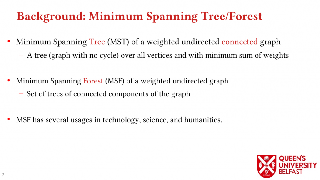
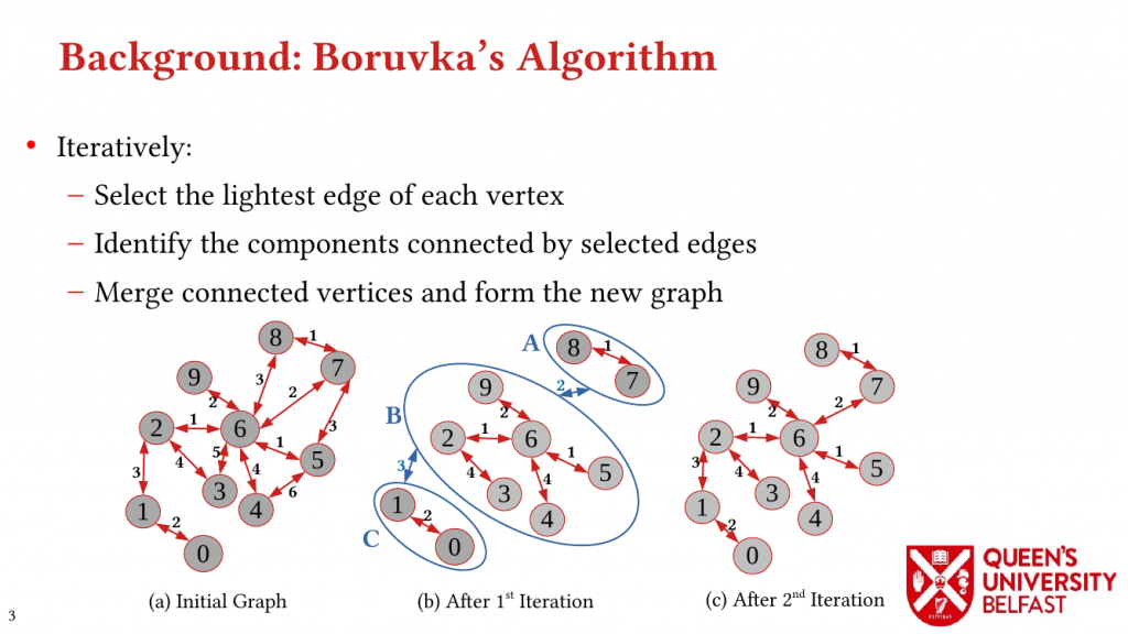
MASTIFF: Structure-Aware Minimum Spanning Tree/Forest – ICS’22

36th ACM International Conference on Supercomputing 2022
June 27-30, 2022
Acceptance Rate: 25%

DOI: 10.1145/3524059.3532365
Authors’ Copy (PDF Format)

The Minimum Spanning Forest (MSF) problem finds usage in many different applications. While theoretical analysis shows that linear-time solutions exist, in practice, parallel MSF algorithms remain computationally demanding due to the continuously increasing size of data sets.

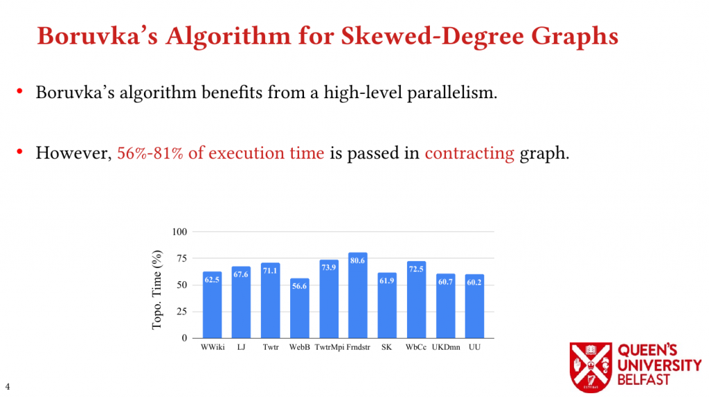
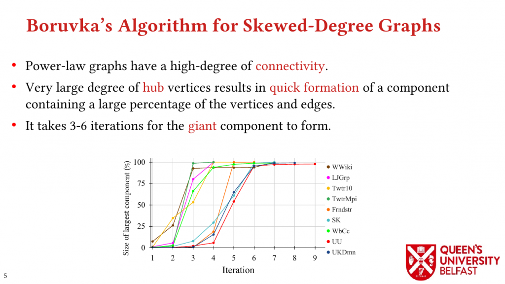
In this paper, we study the MSF algorithm from the perspective of graph structure and investigate the implications of the power-law degree distribution of real-world graphs
on this algorithm.

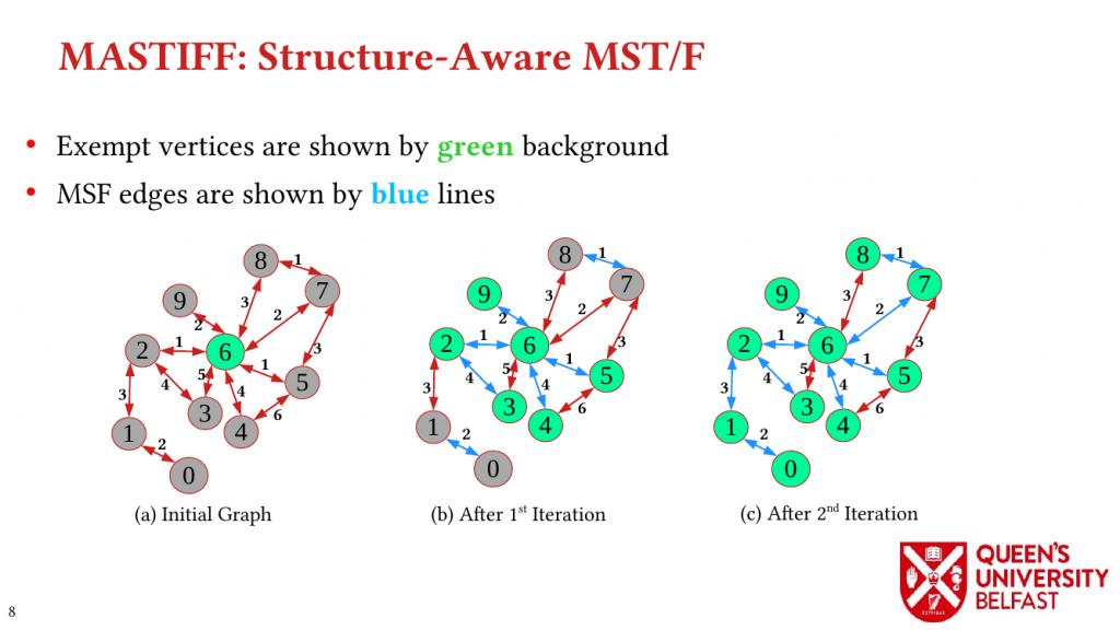
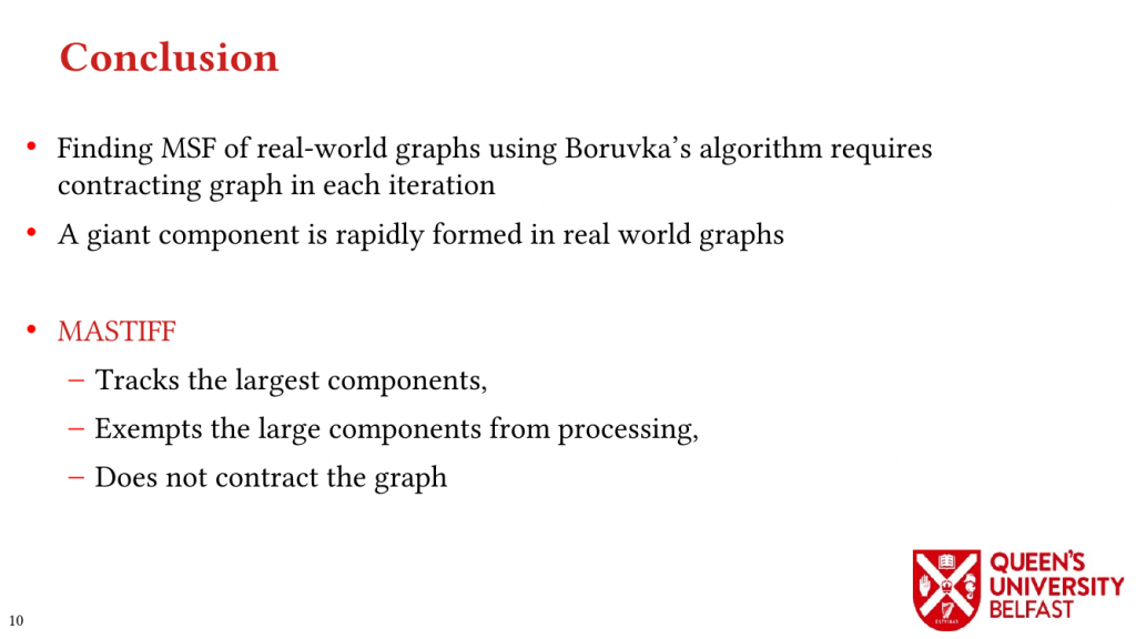
We introduce the MASTIFF algorithm as a structure-aware MSF algorithm that optimizes work efficiency by (1) dynamically tracking the largest forest component of each graph component and exempting them from processing, and (2) by avoiding topology-related operations such as relabeling and merging neighbour lists.

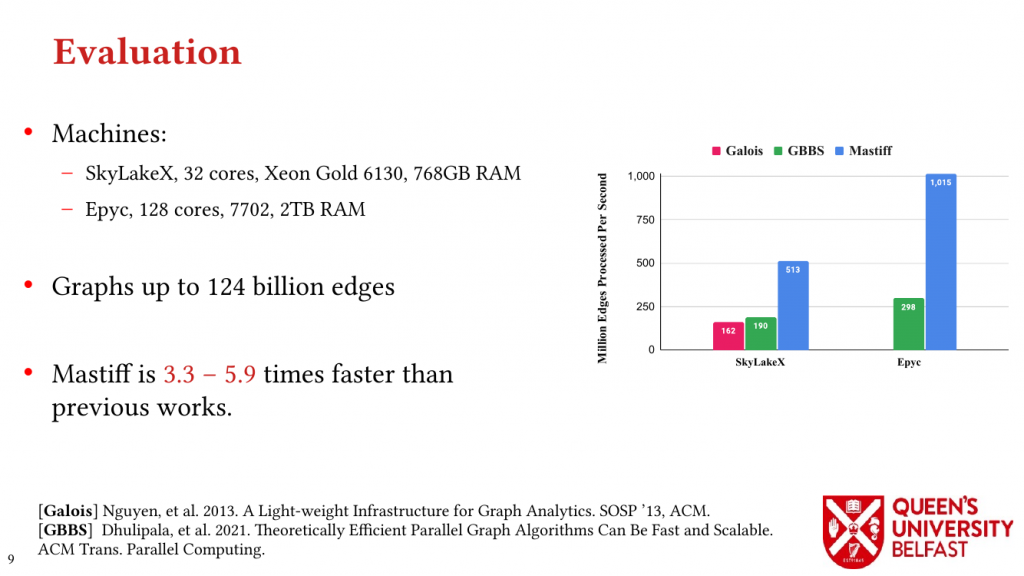
The evaluations on 2 different processor architectures with up to 128 cores and on graphs of up to 124 billion edges, shows that Mastiff is 3.4–5.9× faster than previous works.

Code Availability
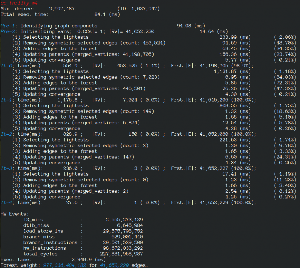
The source-code of MASTIFF is available on LaganLighter Repository (alg3_mastiff.c and msf.c files). A sample execution of this source code for “Twitter-MPI” graph is shown in the following:

BibTex

@INPROCEEDINGS{10.1145/3524059.3532365,
author = {Koohi Esfahani, Mohsen and Kilpatrick, Peter and Vandierendonck, Hans},
title = {{MASTIFF}: Structure-Aware Minimum Spanning Tree/Forest},
year = {2022},
isbn = {},
publisher = {Association for Computing Machinery},
address = {New York, NY, USA},
url = {https://doi.org/10.1145/3524059.3532365},
doi = {10.1145/3524059.3532365},
booktitle = {Proceedings of the 36th ACM International Conference on Supercomputing},
numpages = {13}
}

LaganLighter

Related Posts

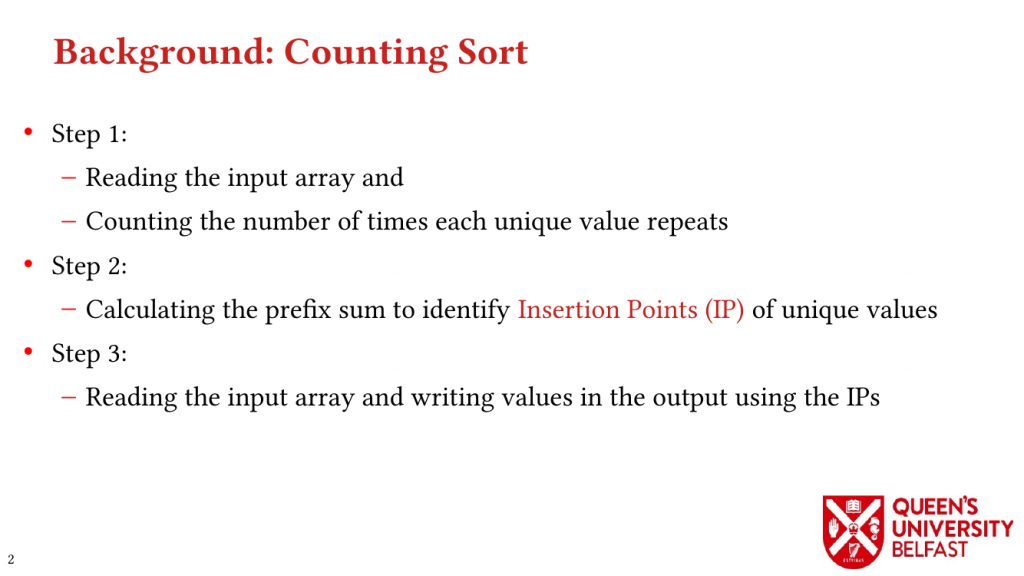
SAPCo Sort: Optimizing Degree-Ordering for Power-Law Graphs – ISPASS’22 (Poster)

2022 IEEE International Symposium on Performance Analysis of Systems and Software (ISPASS 2022)
May 22-24, 2022

DOI: 10.1109/ISPASS55109.2022.00015

Authors’ Copy (PDF)

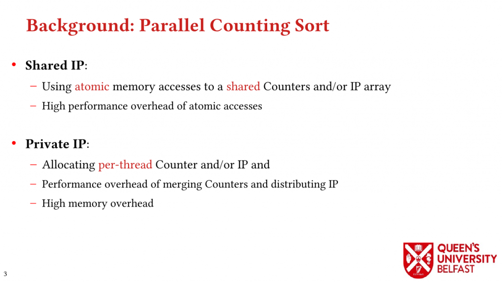
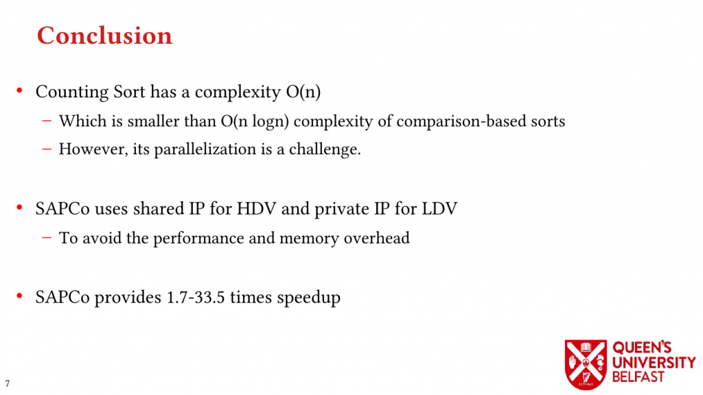
While counting sort has a better complexity than comparison-based sorting algorithms, its parallelization suffers from high performance overhead and/or has a memory complexity that depends on the numbers of threads and elements.

In this paper, we explore the optimization of parallel counting sort for degree-ordering of real-world graphs with skewed degree distribution and we introduce the Structure-Aware Parallel Counting (SAPCo) Sort algorithm that leverages the skewed degree distribution to accelerate sorting.

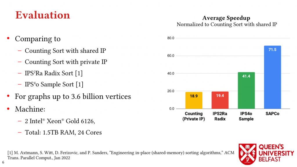
The evaluation for graphs of up to 3.6 billion vertices shows that SAPCo sort is, on average, 1.7-33.5 times faster than state-of-the-art sorting algorithms such as counting sort, radix sort, and sample sort.

For a detailed explanation of the algorithms, please refer to Chapter 5 of the On Designing Structure-Aware High-Performance Graph Algorithms thesis.

BibTex

@INPROCEEDINGS{10.1109/ISPASS55109.2022.00015,
  author={Koohi Esfahani, Mohsen and Kilpatrick, Peter and Vandierendonck, Hans},
  booktitle={2022 IEEE International Symposium on Performance Analysis of Systems and Software (ISPASS)}, 
  title={{SAPCo Sort}: Optimizing Degree-Ordering for Power-Law Graphs}, 
  year={2022},
  volume={},
  number={},
  pages={},
  publisher={IEEE Computer Society},
  doi={10.1109/ISPASS55109.2022.00015}
}

Code Availability
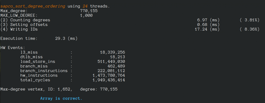
The source-code of SAPCo is available on LaganLighter Repository (alg1_sapco_sort.c and relabel.c files). A sample execution of this source code for “Twitter-MPI” graph is shown in the following:


LaganLighter

Related Posts

LOTUS: Locality Optimizing Triangle Counting – PPOPP’22

27th ACM SIGPLAN Annual Symposium on Principles and Practice of Parallel Programming (PPoPP 2022)
April 2-6, 2022
Acceptance Rate: 31%

DOI: 10.1145/3503221.3508402

Authors’ Copy (PDF Format)

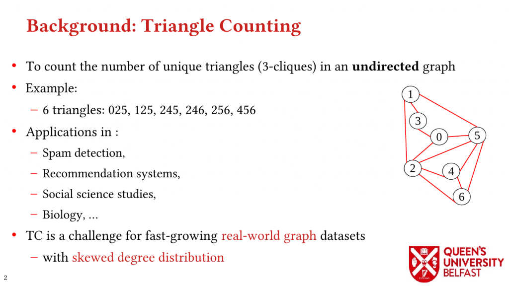
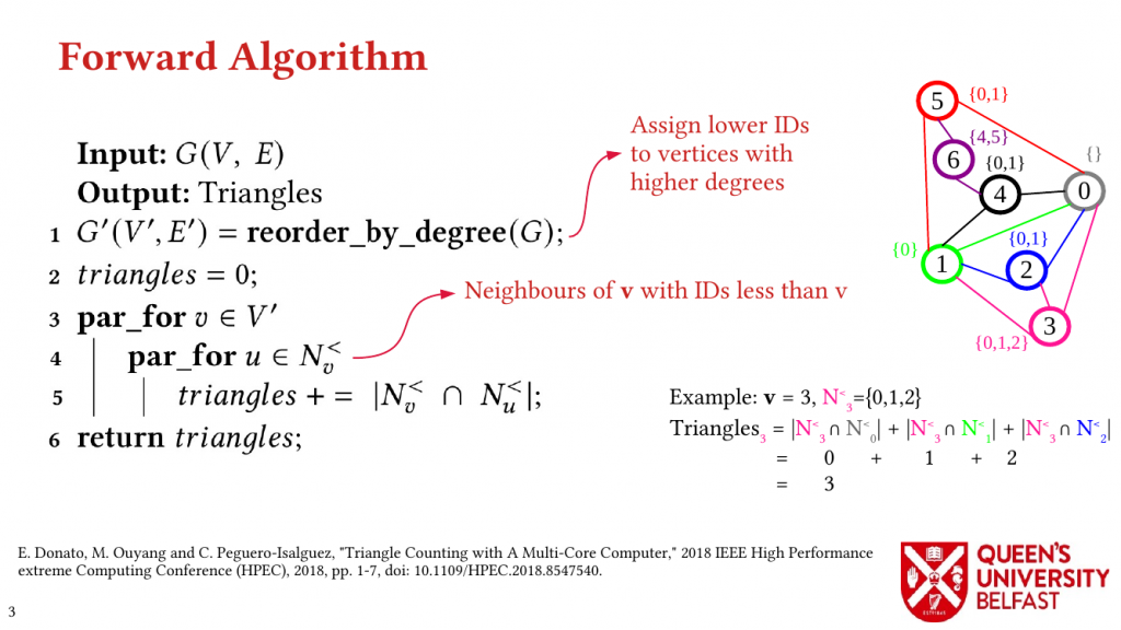
Triangle Counting (TC) is a basic graph algorithm and is widely used in different fields of science, humanities and technology. The great size of real-world graphs with skewed degree distribution is a prohibiting factor in efficient TC.

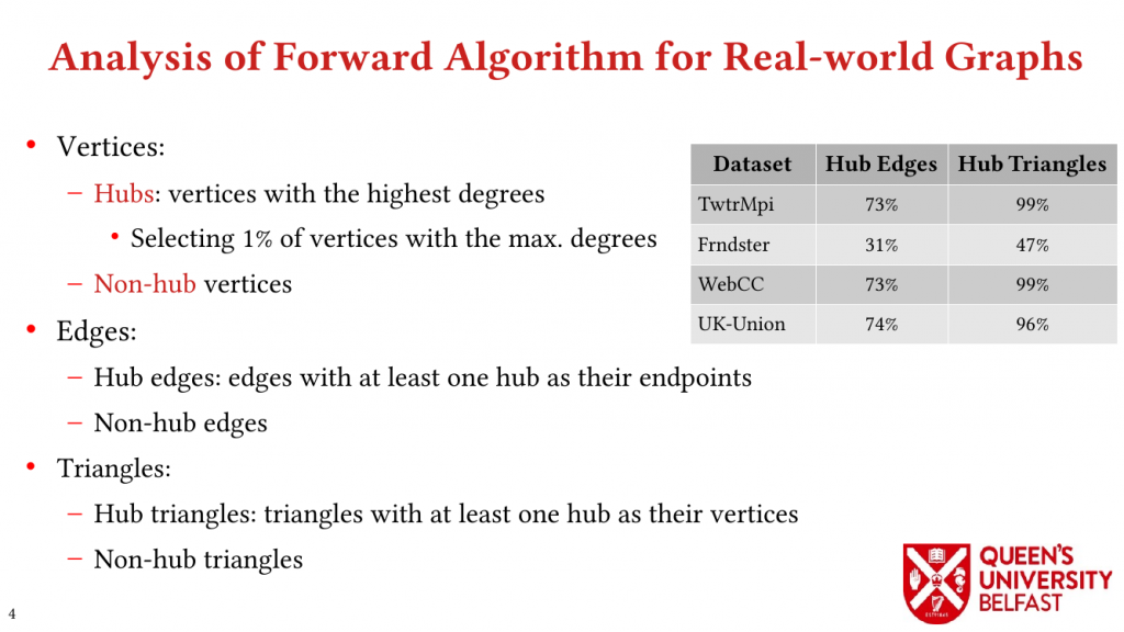
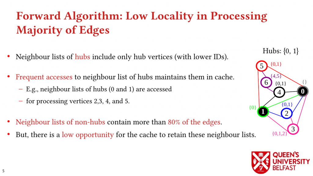
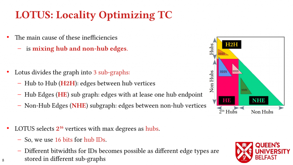
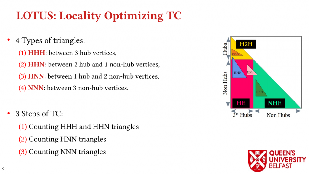
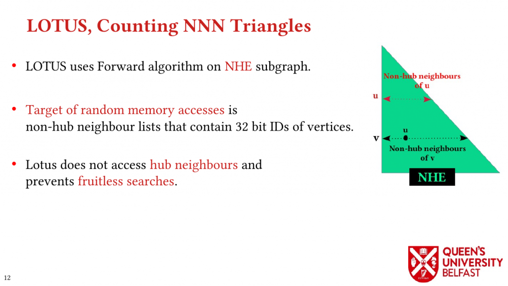
In this paper, we study the implications of the power-law degree distribution of graph datasets on memory utilization in TC and we explain how a great percentage of triangles are formed around a small number of vertices with very great degrees (that are called hubs).

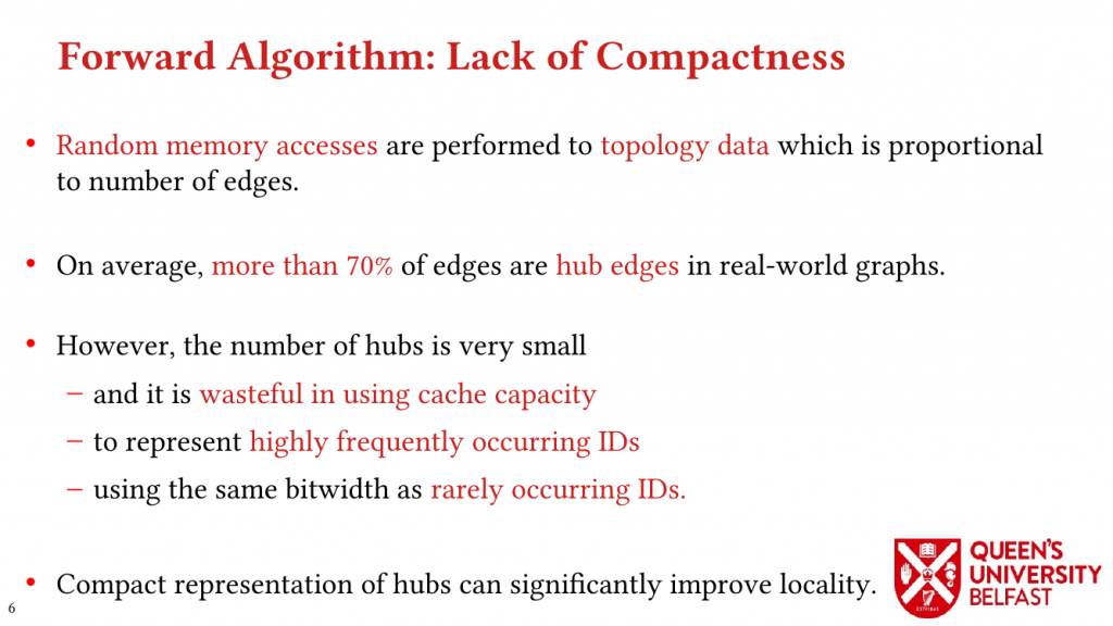
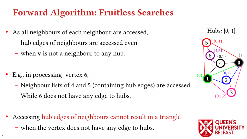
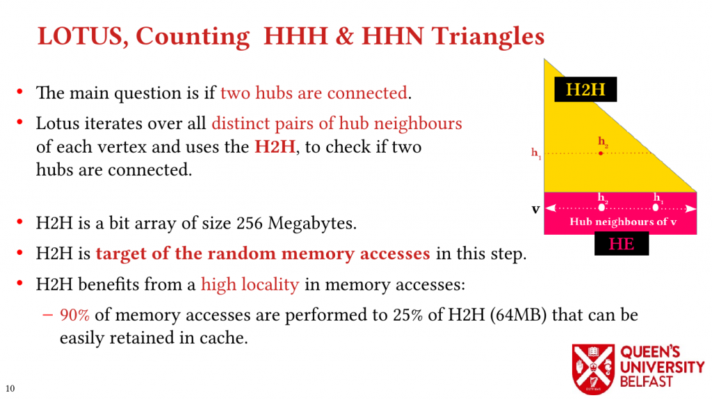
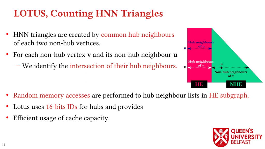
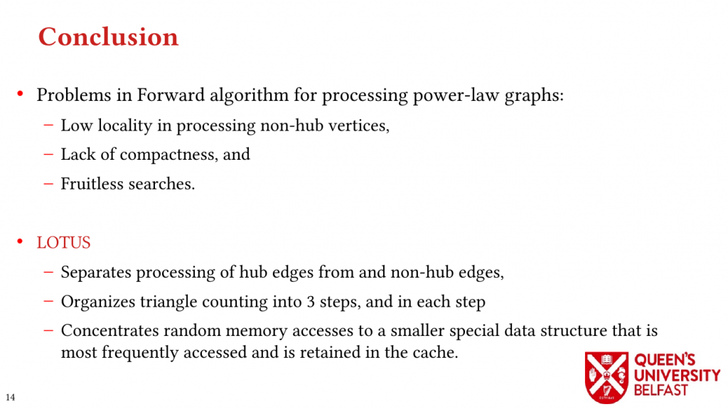
Using these novel observations, we present the LOTUS algorithm as a structure-aware and locality optimizing TC that separates counting triangles formed by hub and non-hub edges. Lotus introduces bespoke TC algorithms and data structures for different edges in order to (i) reduce the size of data structures that are target of random memory accesses, (ii) to optimize cache capacity utilization, (iii) to provide better load balance, and (iv) to avoid fruitless searches.

To provide better CPU utilization, we introduce the Squared Edge Tiling algorithm that divides a large task into smaller ones when the size of work for each edge in the neighbour-list depends on the index of that edge.

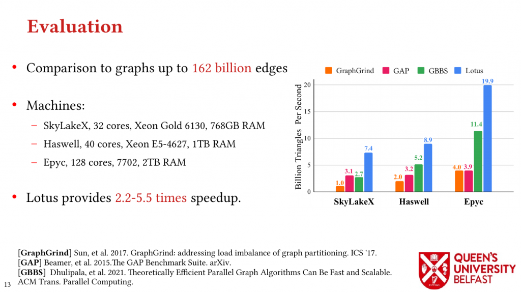
We evaluate the Lotus algorithm on 3 different processor architectures and for real-world graph datasets with up to 162 billion edges that shows LOTUS provides 2.2-5.5 times speedup in comparison to the previous works.

  • LOTUS: Locality Optimizing Triangle Counting
  • LOTUS: Locality Optimizing Triangle Counting
  • LOTUS: Locality Optimizing Triangle Counting - Forward Algorithm
  • LOTUS: Locality Optimizing Triangle Counting - Analysis of Forward Algorithm
  • LOTUS: Locality Optimizing Triangle Counting - Analysis of Forward Algorithm
  • LOTUS: Locality Optimizing Triangle Counting - Analysis of Forward Algorithm
  • LOTUS: Locality Optimizing Triangle Counting - Analysis of Forward Algorithm
  • LOTUS: Locality Optimizing Triangle Counting - Lotus Graph Structure
  • LOTUS: Locality Optimizing Triangle Counting -
  • LOTUS: Locality Optimizing Triangle Counting - HHH & HHN
  • LOTUS: Locality Optimizing Triangle Counting - HNN
  • LOTUS: Locality Optimizing Triangle Counting - NNN
  • LOTUS: Locality Optimizing Triangle Counting - Evaluation
  • LOTUS: Locality Optimizing Triangle Counting - Conclusion
  • LOTUS: Locality Optimizing Triangle Counting -
  • LOTUS: Locality Optimizing Triangle Counting -

Code Availability
The source-code will be published soon.

BibTex

@INPROCEEDINGS{10.1145/3503221.3508402,
  author = {Koohi Esfahani, Mohsen and Kilpatrick, Peter and Vandierendonck, Hans},
  booktitle = {27th ACM SIGPLAN Annual Symposium on Principles and Practice of Parallel Programming (PPoPP 2022)},  
  title = {LOTUS: Locality Optimizing Triangle Counting}, 
  year = {2022},
  numpages = {15},
  pages={219–233},
  publisher = {Association for Computing Machinery},
  address = {New York, NY, USA},
  doi = {10.1145/3503221.3508402}
}

LaganLighter

Related Posts

Locality Analysis of Graph Reordering Algorithms – IISWC’21

2021 IEEE International Symposium on Workload Characterization (IISWC’21)
November 7-9, 2021
Acceptance Rate: 39.5%
DOI: 10.1109/IISWC53511.2021.00020

Authors’ Copy (PDF Format)

Graph reordering algorithms try to improve locality of graph algorithms by assigning new IDs to vertices that ultimately changes the order of random memory accesses. While graph relabeling algorithms such as SlashBurn, GOrder, and Rabbit-Order provide better locality, it is not clear how they affect graph processing and different graph datasets , mainly, for three reasons:
(1) The large size of datasets,
(2) The lack of suitable measurement tools, and
(3) Disparate characteristics of graphs.
The paucity of analysis has also inhibited the design of more efficient RAs.

This paper introduces a number of metrics and tools to investigate the functionality of graph reordering algorithms and their effects on different real-world graph datasets:
(1) We introduce the Cache Miss Rate Degree Distribution and Degree Distribution of Neighbour to Neighbour Average Distance ID (N2N AID) to show how reordering algorithms affect different vertices,
(2) We introduce the Effective Cache Size as a metric to measure how much of cache capacity is used by reordered graphs for satisfying random memory accesses,
(3) We introduce the Assymetricity Degree Distribution and Neighbourhood Decomposition to explain the composition of neighbourhood of vertices to explain structural differences between web graphs and social networks.
(4) We investigate the effects of the structure of real-world graphs on the locality and performance of traversing graphs in pull and push directions by introducing Push Locality and Pull Locality.

Finally, we present improvements to graph reordering algorithms and propose other suggestions based on the new insights and features of real-world graphs introduced by this paper.

BibTex

@INPROCEEDINGS{10.1109/IISWC53511.2021.00020,
  author={Koohi Esfahani, Mohsen and Kilpatrick, Peter and Vandierendonck, Hans},
  booktitle={2021 IEEE International Symposium on Workload Characterization (IISWC'21)},  
  title={Locality Analysis of Graph Reordering Algorithms}, 
  year={2021},
  volume={},
  number={},
  pages={101-112},
  publisher={IEEE Computer Society},
  doi={10.1109/IISWC53511.2021.00020}
}

Related Posts

LaganLighter

Thrifty Label Propagation: Fast Connected Components for Skewed-Degree Graphs – IEEE CLUSTER’21

IEEE CLUSTER 2021

IEEE CLUSTER 2021
7-10 September

Acceptance rate: 29.4%

DOI: 10.1109/Cluster48925.2021.00042
IEEE Xplore
PDF Version (Authors’ Copy)

Thrifty introduces four optimization techniques to Label Propagation Connected Components:

1) Unified Labels Array accelerates label propagation by allowing the latest label of each vertex to be read in processing other vertices.

2) Zero Convergence optimizes work-efficiency in the pull iterations of Label Propagation by skipping converged vertices.

3) Zero Planting selects the best start propagating point and increases the convergence rate and removes pull iterations that are required for the lowest label to reach the core of graph.

4) Initial Push technique makes the first iteration work efficient by skipping processing edges of vertices that probability of convergence is very small.

Based on these optimizations, Thrifty provides 1.4✕ speedup to Afforest, 6.6✕ to Jayanti-Tarjan, 14.3✕ to BFS-CC, and 25.0✕ to Direction Optimizing Label Propagation.

  • Thrifty Label Propagation: Fast Connected Components For Skewed Degree Graphs
  • Thrifty Label Propagation: Outline
  • Thrifty Label Propagation: Background
  • Thrifty Label Propagation: Background
  • Thrifty Label Propagation: Background
  • Thrifty Label Propagation
  • Thrifty Label Propagation: Unified Labels Array
  • Thrifty Label Propagation: Unified Labels Array
  • Thrifty Label Propagation: Zero Convergence
  • Thrifty Label Propagation: Zero Convergence
  • Thrifty Label Propagation: Zero Planting
  • Thrifty Label Propagation: Zero Planting
  • Thrifty Label Propagation:  Initial Push
  • Thrifty Label Propagation:  Evaluation
  • Thrifty Label Propagation:  Evaluation
  • Thrifty Label Propagation:  Evaluation
  • Thrifty Label Propagation:  Conclusion
  • Thrifty Label Propagation:  Thanks
  • Thrifty Label Propagation:  A Gift from QUB


Code Availability
The source-code of Thrifty is available on LaganLighter Repository (alg2_thrifty.c and cc.c files). A sample execution of this source code for “Twitter-MPI” graph is shown in the following:


Bibtex

@INPROCEEDINGS{10.1109/Cluster48925.2021.00042,
  author={Koohi Esfahani, Mohsen and Kilpatrick, Peter and Vandierendonck, Hans},
  booktitle={2021 IEEE International Conference on Cluster Computing (CLUSTER)}, 
  title={Thrifty Label Propagation: Fast Connected Components for Skewed-Degree Graphs}, 
  year={2021},
  volume={},
  number={},
  pages={226-237},
  publisher={IEEE Computer Society},
  doi={10.1109/Cluster48925.2021.00042}
}

Related Posts