Our friends at OpenDataNI have been busy securing some fantastic spatial data sets for public use. in particular LiDAR surface elevation data collected by various NI Government Departments over the last 12 years. I’ve covered LiDAR technology in a previous post showing how it is used in our research here at SNBE, but I thought it might be useful to show how you to can, process, visualise and interrogate the data using free Geographical Information Systems (GIS) software applications.
(This blog QGIS 3.10 – Long Term Release)
Spurred on by the release of Environment Agency England LiDAR elevation data, OpenDataNI has collated and uploaded LiDAR data from the Department of Infrastructure (Rivers and Flooding/TransportNI) and the Department of Communities (Historic Environment Division). At this stage it is important to note that the LiDAR survey data covered in this blog was originally collected independently and for different output roles; flood prediction and mapping, and identification, analysis and management of archaeological landscapes. As a result the output data sets do not cover the whole of NI and are at different ground resolutions (Rivers c1m and Historic c0.2m). For example researchers are better able to identify small archaeological surface features at higher resolutions (<1m) but modelling a river basin and catchment for flood flow prediction does not necessarily require these very high resolutions (>1m).
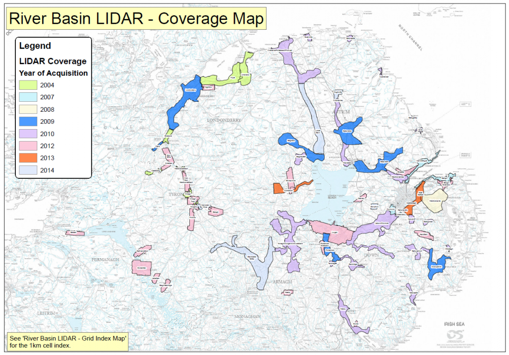
River Basin Coverage 2004 -2014 (OpenDataNI)
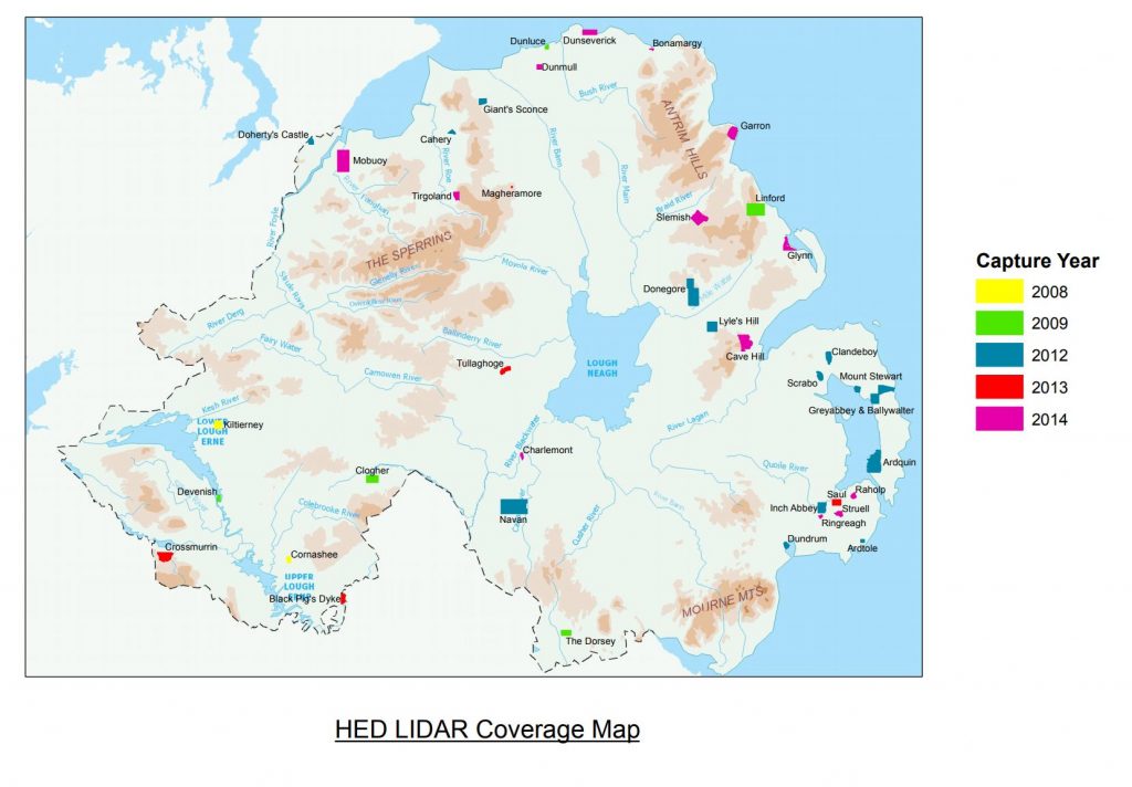
Historic Division Coverage 2008 - 2014 (OpenDataNI)
Ok so you have identified the liDAR coverage area you area interested in and have downloaded the data from OpenDataNI (be careful LiDAR data is large!). What can you do with it? How can we visualise and analyse the surface elevation that has been surveyed? I’m lucky here at QUB as a GI Scientist, we have lots of great ‘commercial’ GIS applications we can access to for teaching and Research (ESRI). But what if you want to have a go at finding a new geological or archaeological surface feature that has yet to be mapped! Thankfully there are some great free and ‘Open Source’ GIS that you can install at home! One of the most widely used free GIS packages is QGIS. Download and install to your favourite OS flavour (Win/OSX/Linux). I’m using the 3.4 version for this blog post.
QGIS Web and Download Site - www.qgis.org
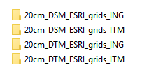
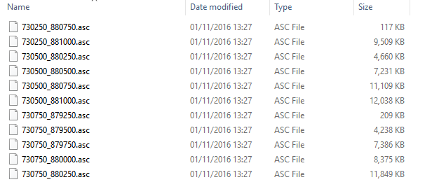
Once installed prepare your LiDAR data (I’m using the Cave Hill data in this example – 2014). You will notice that the data has been downloaded as one large compressed ‘ZIP’ file, you need to extract this file to access the LiDAR data. Once extracted, delete the downloaded ZIP file to save space. Open the data folder, in this case we have 4 sub-folders, 2x 0.2m (20cm) resolution Digital Surface Model data sets and 2x 0.2m (20cm) Digital Terrain Model data sets. [I’ve covered the difference between DSM and DTM and how they are created in the previous blog]. We will work with the DTM Irish National Grid (ING) coordinate system data. This data has been projected to Irish National Grid coordinates and has been processed with vegetation and buildings removed (anthropocentric filtering), helping us to see the ground surface below. The DSM includes all the LiDAR data and is useful for mapping tree and building heights! The Irish Transverse Mercator (ITM) projection has been applied to the other data copies and is common in the Republic of Ireland.
LiDAR folders and data files (CG GIS QUB)
Coordinate Reference System
Before we ‘build’ the LiDAR data surface we will set the project Map Projection or Coordinate Reference System (CRS) to Irish Grid. Click on the CRS button on the bottom right of the QGIS window to activate the CRS popup. In the ‘Filter’ box, type ‘Irish‘ and select TM75 / Irish Grid – Traverse Mercator 1975 is the current coordinate system for Northern Ireland and supported by the Ordnance Survey of Northern Ireland.
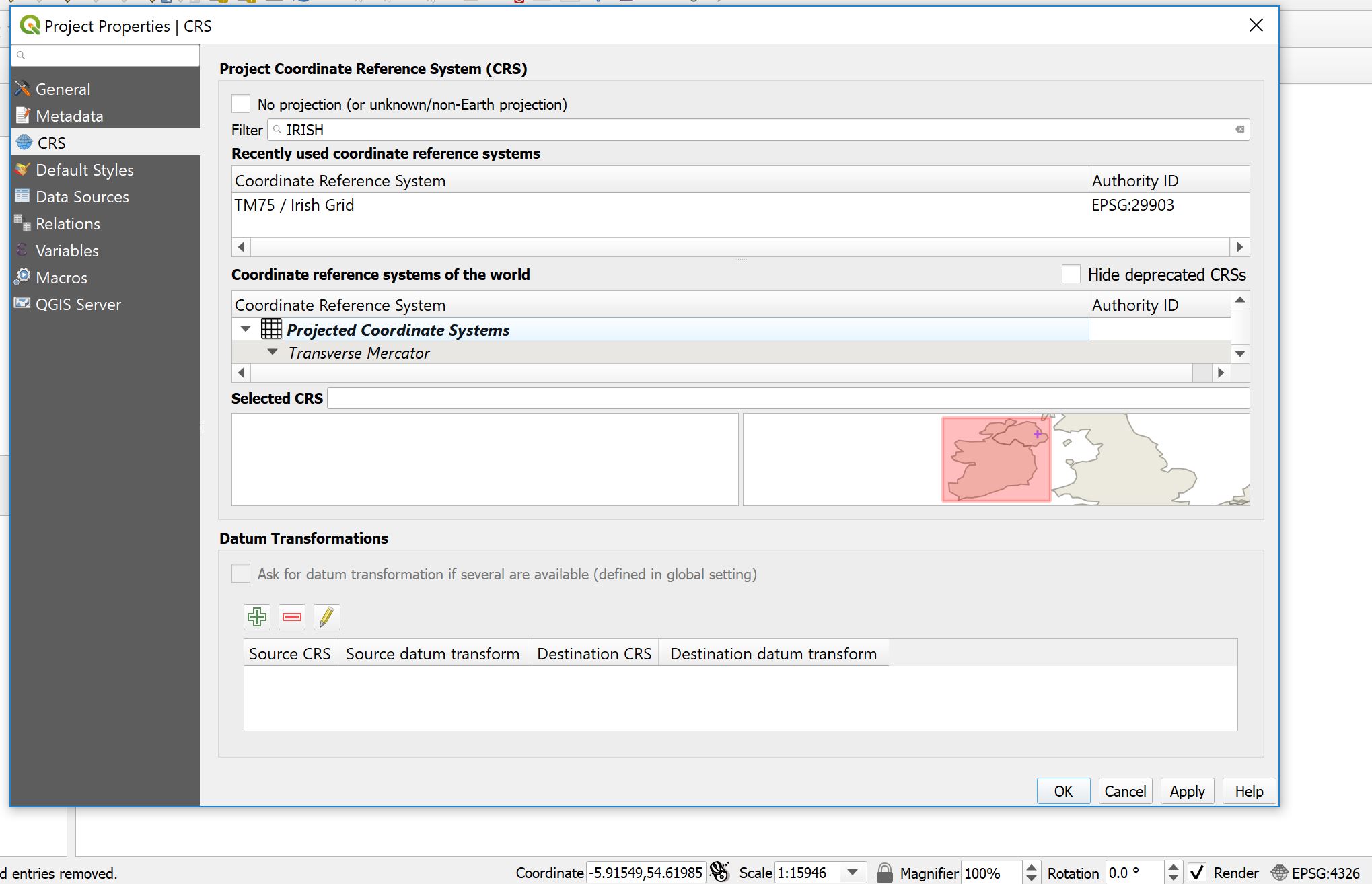
CRS Popup (CG GIS QUB)
Build the LiDAR VRT Surface
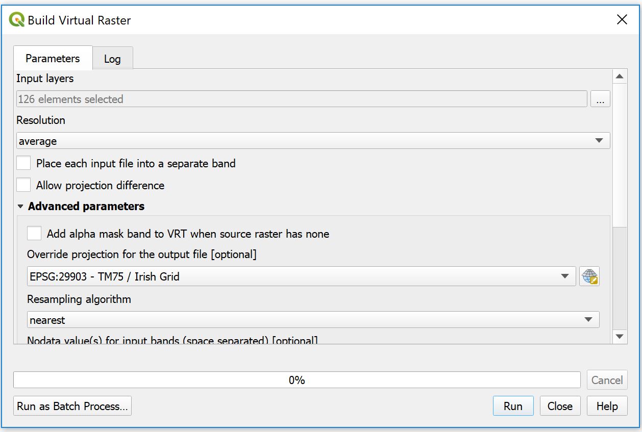
The LiDAR surface elevation data is stored as ASCII format files (.asc), a Raster grid format file. Each tile covers a fixed area depending how the data has been segmented, with 1000’s of 20cm cells recording height. The tiles are seamless with joining tiles (‘edge to edge’). We could add the individual tiles to the GIS as required but we are going to use a more productive virtual ‘Mosaicing’ process to create a seamless, continuous elevation surface to analyse. Open QGIS desktop and from the menu select Raster > Miscellaneous > Build Virtual Raster. (VRT)
[Make sure Menu > Plugins > Installed > Processing is checked]
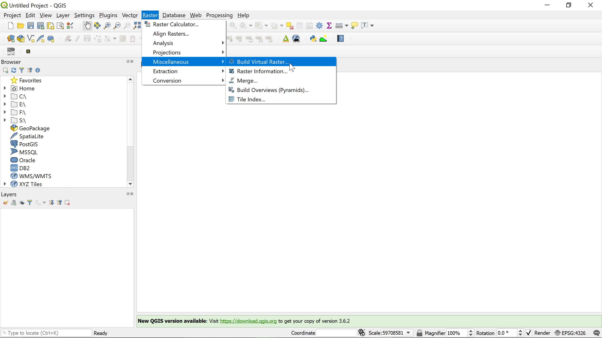
QGIS Build Virtual Raster (CG GIS QUB)
In the ‘Input Layers‘ box click on the open folder button (…) to open the ‘Multiple Selection‘ popup and click on ‘Add Files‘ and browse to the downloaded and extracted LiDAR folder that we are going to mosaic (eg. 20cm_DTM_ESRI_grids_ING). Order the files based on ‘type’ and using the shift key on your keyboard select all the .asc files together and click Open. In the Multiple Selection popup a list of the selected files will be detailed on the left. Click OK to add the selection to the Input Layers, you should have 126 files (elements) added if using the Cave Hill raster tile layers. Finally uncheck the ‘Place each input into a separate band‘ option and leave all options as the defaults.
As an optional step in the ‘Advanced Parameters‘ and to insure the output CRS is Irish Grid you can select TM75 / Irish Grid from the ‘Override Projection..‘ drop down option. Finally click Run to start the VRT process!
QGIS Build Virtual Raster (CG GIS QUB)
Depending on the spec of your computer it may take a few minutes for the process to complete and display the new VRT mosaiced dataset.
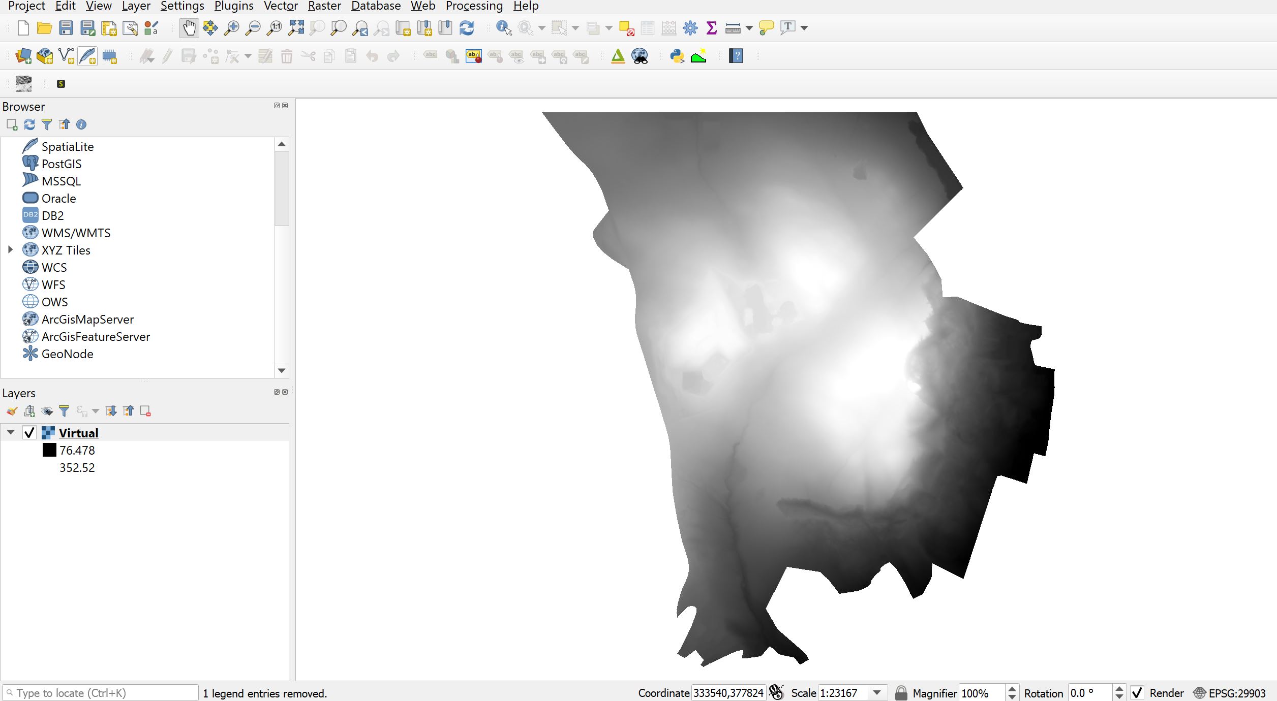
Completed Cave Hill LiDAR layer Mosaic in QGIS (CG GIS QUB)
QGIS will now display the LiDAR mosaic as a ‘Grey Scale’ colour ‘render’ by default, and list the new VRT layer in the ‘Layer Panel’ on the left. The grey scale Raster layer displays the elevation range (76m – 352m) as low (black) to high (white). Elevation is metres above sea level, in this case Belfast Lough. This colour render can be changed in the layer properties (Symbology) if you want to experiment!
We now have a continuous elevation surface at 0.2m resolution. Unfortunately this is not a very informative visualisation at the moment, even if you zoom in to the data! Thankfully the GIS has a few neat tools to help out! First we will create a Hillshade Model, the ‘go to’ technique for a first look at a LiDAR elevation surface. A hillshade is a grayscale representation of the surface, with the sun’s relative position taken into account to calculate and model shadows (shading) on the elevation surface. We can set the elevation of the sun above the horizon (Altitude) and the compass bearing (Azimuth). This process creates ‘virtual shadows’ that can help outline surface topography including geological, geomorphological and archaeological features. Buy experimenting with different sun orientation settings we can help identify features that are very difficult to see in the DTM surface alone.
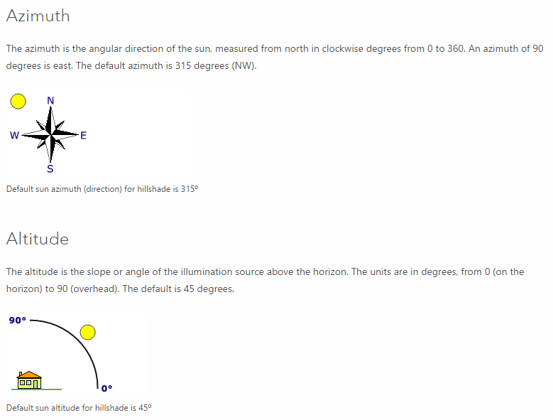
Azimuth and Altitude (ESRI.com)
To generate a Hillshade surface In QGIS, from the Menu select Raster > Analysis > Hillshade, with the Cave Hill VRT selected as the Input Layer (this will create a temporary Hillshade layer unless you specify a name and folder location to save to). The default settings in QGIS for the Hillshade Sun elevation (altitude) is 40 degrees and the Azimuth (compass) is 315 degrees. These can be changed to model differing Sun angles.
Click Run to start the analysis. After processing completes the new layer will be added to QGIS!
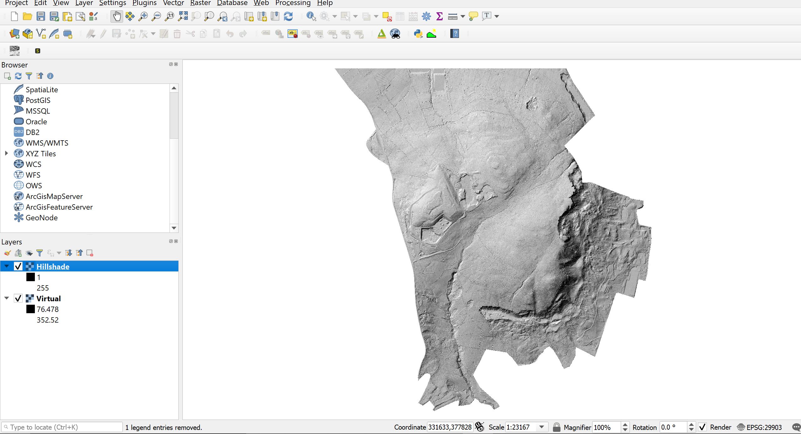
Hillshade Layer in QGIS (CG GIS QUB)
The Hillshade shows a shaded ‘greyscale ‘colour value range between 0 and 200 (black to white) and does not represent the surface elevation. Because we have used a very high resolution DTM (20cm) we should be able to see features as small as 20cm on the ground! Use the Zoom and Pan tools to explore the new topography layer and examine all the ‘humps n’ bumps’ not normally visible! If you tick off [x] the LiDAR VRT surface in the layer below, the map will render faster.
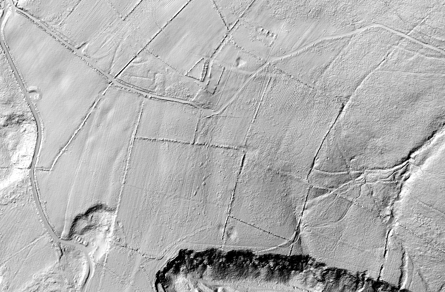
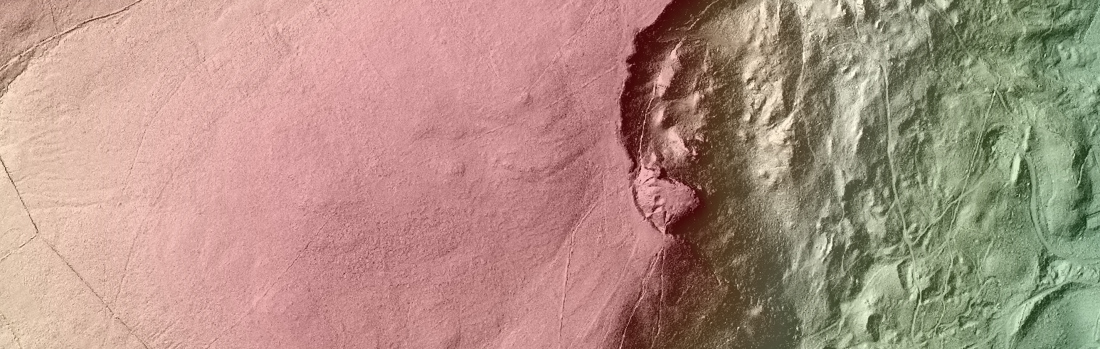
Hillshade Layer in QGIS. Zoomed in showing shading relief and surface features. 'Relic farmland' on the South Slope. (CG GIS QUB)
We can also add background Aerial Imagery (Orthophotos) and mapping to help with our geography and landscape analysis using the ‘XYZ Tiles’ layer in QGIS. In the ‘Browser Pane’ layer list double click on the XTZ Tiles layer to open the mapping options. In this case click Google Satellite or Bing VirtualEarth to add background aerial imagery. These new layers will be added to the Layer list and you can switch the layers on an off (x) to compare the Hillshade and ‘current’ aerial images of the location, or move layers in the list to rearrange their order. You need a web connection to connect to background mapping. Here are some other XYZ Tile options.
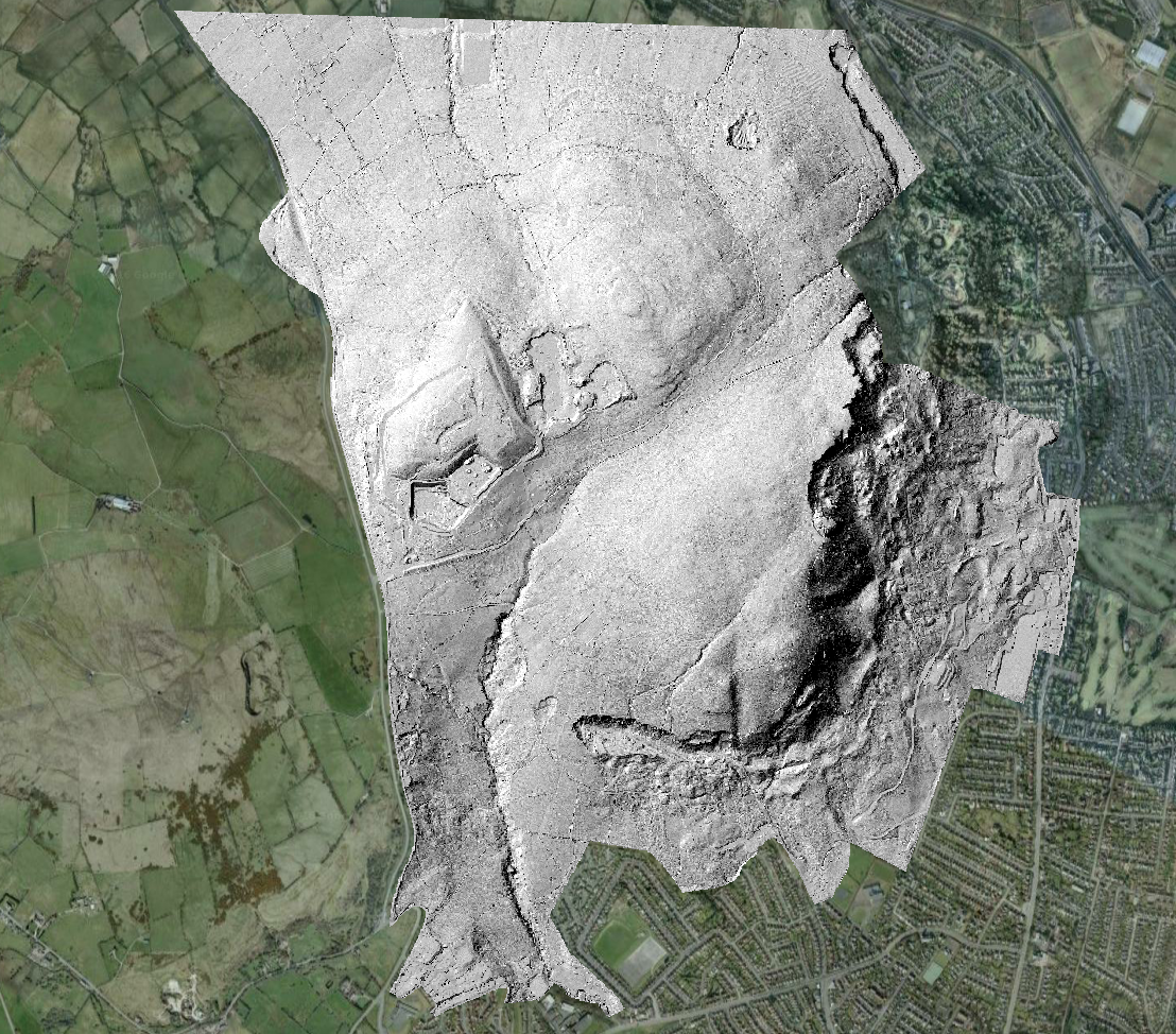
Hillshade Layer and XYZ Tile Google 'Satellite' Maps background imagery. (CG GIS QUB)
It is also possible to set the ‘Transparency’ of layers to aid visualisation. Double click over the layer in the list to open the Properties Window. Combining a new colour ramp for the elevation data and setting the transparency of the Hillshade is a great way to visualise both the LiDAR elevation data and Hillshade together and can help interpret surface features. Open the LiDAR Data layer Properties window (double click on layer) and change the Render Type to Singleband pesudocolour. In the Colour drop down below select a colour ramp, RdYlGn (Red Yellow Green) works well and check the Invert box. Click OK. Double click on the Hillshade layer and set the layer transparency to 30% and click OK.
Save your QGIS LiDAR project and start searching for surface features! 🙂
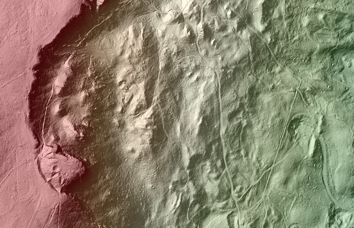
Hillshade Layer and LiDAR DTM overlay. Large landslide features, East face of Cave Hill. (CG GIS QUB)
View the LiDAR surface in 3D!
Finally we can use the 3D viewer built into QGIS to visualise the LiDAR surface and your visualisation. 3D map views are useful way to add a more realistic ‘context’ to you GIS work and can bring extra understanding to your data that may not be apparent in more ‘traditional’ 2D views.
QGIS uses a dedicated 3D viewer with mouse and Tool navigation. Views are based on the active checked/symbolised data layer in the Layer Pane and can be exported as images for lots of uses including sharing cool landscape features on social media platforms!
In Menu > View> New 3D Map View
- A new 3D Popup will be generated rendering your active data in ‘3D’ (The window can be resized)
- If you have an XYZ Tile background layer activated it can take some extra time to render this layer so it might be worth while switching it off until you set things up.
- To limit the data ‘render’ area to the extent of the DTM (Virtual Raster) click on the 3D view configuration tool
 and select the elevation surface you want to use e.g. Virtual Raster / LiDAR DTM.
 - Turn on your XYZ layer in the Layer Pane.
- Use you mouse (left click and roller wheel) to navigate the view or the navigation tools in the 3D window.
- You can experiment with the 3D view render resolution (Map tile) and Vertical Scale (Vertical exaggeration). Multiplying the height values (Z) by a scale value e.g. 1.5. This will ‘exaggerate’ the 3D height of the DTM surface in the view making it easier to see ‘low elevation’ surface features, but don’t go to crazy!
- To export an image of the 3D view > Save as Image tool
 and share your 3D visualisation!
 - If you are interested in generating a 3D animation and movie checkout this tutorial.
Newry Valley DTM in 3D Viewer. CG
Congrats! You are now a LiDAR analyst 🙂
Experiment with other [Terrain] Analysis operations (slope, aspect etc) and other LiDAR data from OpenDataNI!
Checkout my Hillshade analysis results here in 2d and as a 3d view. Thanks for reading!
CG.
About the Author:
Conor is the Geographical Information Systems (GIS) Research Officer at the School of The Natural and Built Environment, Queen’s University Belfast and manages a dedicated GIS Research and Teaching lab with colleagues Lorraine Barry, Jennifer McKinley and William Megarry. An active GI Educator and Researcher for over 15yrs , STEM Ambassador and a member of the The Society of Chartered Surveyors Ireland and Royal Institution of Chartered Surveyors with interests in Geomatics, Geodesy, Digital Survey, Remote Sensing, Web Mapping and spatial data collection and analysis utilising UAV/Drone technologies. When not working with, or collecting Spatial Data Conor is a very keen Mountain biker (with a GPS attached)!
Fantastic work. Easy to understand, step by step instructions really help. Glad to have found this. Many thanks.
Thanks Sebastian,
It would be great to see how you are using the LiDAR data.
Conor.
Such a brilliant tutorial. I’m now (finally) able to upload the LiDAR data into QGIS.
C
Thanks Chris. We wanted to show that Public LiDAR is accessible using Open GIS Software. 🙂
Great turtorial Conor thanks!
James
I like the helpful info you provide in your articles. I will bookmark your weblog and check again here regularly.
Wonderful tutorial and timely for my project. Thank you for the clear and up to date tutorial!
Erik
We appreciate that! Hope to keep providing good information 🙂
Conor.
I hope you can help. I live in Scotland and have been using lidar data to create data for my golf course and others to allow users of the software “TGC2019”. This is a golf simulator package that allows users to play golf in a simulator.
Having created and published a few courses, A golfer in NI asked me if I could help him realise his course at Castledawson Moyola park golf club. From one of your maps, it looks like Lidar is available for this area.
The package I use needs a laz file.
Do you know if there is any Laz data for this area or data I can convert to Laz for that area?
Any help appreciated
David
Hi David, did you every get a response about this? I want to recreate Strabane Golf club in Co. Tyrone for GSPRO. Any help would be greatly appreciated.