By Jacob Garby
Motivation
Optimising deep learning has become a hugely important task in computer science. The networks themselves have countless applications, including image and handwriting recognition, data clustering and prediction, and even medical diagnosis assistance. Training requires feeding a large amount of data into an algorithm, producing a model which gradually becomes better and better at a desired task.
A huge number of calculations are needed to carry out this training, but predictions may be made with relatively little computation once the model is trained sufficiently. Over time, our computers have become faster. This allows neural network training to take less time, and hence develop more accurate models. The increase in raw processor clock speed has plateaued though, since it has become inefficient (in terms of heat dissipation) to run the CPUs at higher and higher clock speeds, despite significant advances in transistor process efficiency.
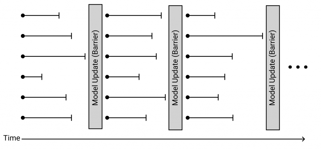
Due to this bottleneck, there has for a long time been widespread research into parallel computing. Using a number of processors which work together to solve some task can yield significant performance improvements. In the context of deep learning, the task is training a deep neural network. Starting from an initial randomised model, each processor may, concurrently, determine (based on a small and individual portion of the whole set of training data) how it thinks the model should be altered to be a little bit better. These “suggestions” made by each of the processors can then simply be averaged together and applied. This execution strategy can be represented as follows:

In the above, the grey rectangles represent the times at which the model is being updated by aggregating the results computed by individual threads of execution. Each thread is represented by a line. The circle-end of each line represents the point in time at which the thread begins, by selecting a portion of the dataset to work on. The line segment represents the time it takes to compute its update based on this data. This update is known as a gradient. The vertical bar at the end of each line segment represents the point in time at which that thread has finished, and is ready for its gradient to be incorporated into the model. Note that the entire execution is, in this manner, divided into a number of training “rounds”.
This strategy, in which threads must wait for each other before beginning subsequent rounds, is referred to as being synchronous.
Why Synchronous Parallelism Isn’t Good Enough
It can be observed in the above diagram that at a given point in time, some threads may not be doing anything. This happens when certain threads finish a training round faster than others. This reduces the speedup in throughput that we could expect from a concurrent algorithm. The threads that take significantly longer to finish are named “stragglers”.
The type of system that we have described so far is a “shared memory” system, which means that all of the threads/processors communicate with each other implicitly through shared direct access to physical memory, as in a standard desktop computer. This can appear as one socket with a number of processing cores, or several such sockets. Another architecture on which parallel processing can run is a “distributed” system, where threads communicate usually via the sending and receiving of messages. These messages can be sent over a network spanning a large geographic area (i.e. the internet) with high latency, or around a large supercomputer. In this context, each thread may run on an individual processing core (as with the sort of shared memory system discussed previously), or on a processing node which itself is a multi-core computer. In each type of system architecture, stragglers may occur for various and overlapping reasons.
In both cases, the data may be divided between the threads in such a way that some must carry out a longer sequence of calculations in order to complete a round. This may be unavoidable, since it isn’t necessarily knowable beforehand which batches of data will take longer.
In both cases (though more prevalent in distributed systems), there may be some degree of processor heterogeneity, i.e. some processors are faster than others. In a shared memory system, this may be the case on CPUs which have a number of “performance” cores and a number of low-power cores. In a distributed system this could also be the case, but also it may actually consist of a number of completely different models of processor.
In a distributed system specifically, latency between machines can play a role in the existence of stragglers. Processors which take longer to communicate with the system coordinator may be able to finish their computations in a similar amount of time to the others, but the additional time taken to fetch a copy of the model (and possibly their batch of data), and to send their gradient back, may result in additional waiting.
The existence of stragglers in a synchronous algorithm like this forces other threads to wait. The more time threads spend doing nothing, the further from optimal the algorithm becomes, in terms of throughput.
Pros and Cons of Asynchronous Parallelism
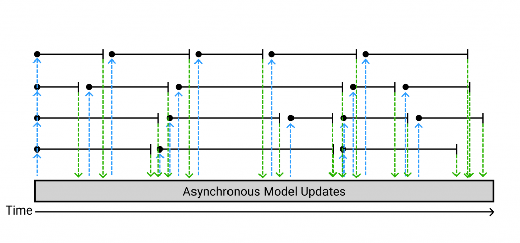
A solution to this is to remove the restriction of synchronicity. This may at first seem trivial — simply allow any thread to start work on new data immediately after finishing one round of computation, and repeating. At the beginning of each training round, each thread has to make itself a copy of the central model, which it bases its training on. And then, after it finishes a round, it just applies its update to back to the global model. Here lies the problem, though: the central model may have, at this point, already been changed by another thread’s update! This execution strategy looks like the following.

The notation is roughly the same as the synchronous diagram, except now we have these blue and green lines which represent threads taking copies of the global model and incorporating their computed gradient into it, respectively. Here it’s easy to see that in almost every case, the model undergoes some updates between a given thread’s “pulls” and “pushes”. Additionally, this is with only four threads. In real applications, hundreds (or even thousands) of threads may be used.
When an update is applied that was calculated based on an outdated view of the model, that update becomes less relevant. The application of gradients which are not relevant to the current state of the model mean that the algorithm can take a far higher number of updates before it reaches the desired accuracy.
This type of execution is known as asynchronous. Its throughput is generally far higher than a comparable synchronous implementation, due to the absence of waiting between training rounds. The trade-off is in model accuracy: even though the throughput may be higher, the program may still take longer to get a model of a similar quality.
Progress and Plans
My research at the moment deals primarily with designing asynchronous execution strategies for training deep neural networks. I’ve been looking into various ways of managing the trade-off between throughput and accuracy.
I’ve been specifically working on algorithms which aim to, at runtime, select the most efficient number of threads, based on intermittent probing of settings. This work is based on the observation that, in many cases, a number of active threads less than the maximum available is optimal in terms of improvement in model accuracy per unit time. The primary challenge here is designing a probing strategy which converges on a performant configuration in as few steps as possible, since time spent probing at non-optimal settings negatively impacts the convergence rate of the overall system.
